29.1 Algorithmic speedups🔗⧉

A direct radius-$k$ blur sums a $(2k+1)\times(2k+1)$ neighborhood for each of $N$ output pixels, costing $O(Nk^2)$. A separable kernel reduces this to $O(Nk)$. A box filter can be computed with running sums at radius-independent cost per output after initialization; a Gaussian can be approximated by a fixed-order recursive filter at $O(N)$ cost. These are different results: the recursive approximation does not compute an arbitrary finite Gaussian kernel exactly.

Algorithmic changes can save arithmetic, memory, or both. Some preserve the operator in exact arithmetic; others trade quality for speed. Keep those categories distinct, and compare against a reference with the same boundary convention. The following techniques complement scheduling rather than replace it.

29.1.1 Precompute and look up: pay once, before the loop🔗⧉

A function of one 8-bit value has only 256 possible inputs. Evaluate it once for each input, store the results, and replace repeated evaluation by a table lookup. This can make an expensive tone curve cheap; Chapter 45.33, Photoshop 1.0, running gives an early implementation example.

A table trades arithmetic for storage and indexed reads. A two-byte input domain already has 65,536 entries, with storage determined by the output type. Lookup cost depends on cache residency and vector support; a small polynomial may run faster than a large table. Even a 256-entry table competes with other data for cache. Measure both forms.

For continuous inputs, tabulate samples and interpolate. State the input range and behavior outside it, and test approximation error between samples, especially near steep curve segments. Rebuilding a table for every frame can erase the saving on small images.

Lookup tables apply to more than one-dimensional tone curves. A function of two unsigned bytes has 65,536 possible input pairs, so it can be tabulated if that storage and access pattern are worthwhile. The table trades repeated arithmetic for memory traffic. A small table that stays near the processor can be attractive; a large table indexed irregularly can lose to recomputation. When the domain is continuous, interpolation between stored samples adds an approximation whose error must be considered separately from the lookup's speed. The older implementations in Chapter 45.33, Photoshop 1.0, running make the arithmetic-saving motivation concrete.

29.1.2 Separability: a 2-D pass for the price of two 1-D passes🔗⧉

A separable kernel factors as $K(u,v)=h(u)g(v)$. Substitution gives

Compute the bracketed horizontal filter first, then filter its result vertically. The work per output falls from $(2k+1)^2$ weighted contributions to $2(2k+1)$. For a $25\times25$ kernel, that is 625 versus 50. Equality assumes the same kernel and compatible boundary extension; floating-point rounding can still differ.

The second pass introduces an intermediate and its memory traffic. A vertical stencil is not automatically contiguous in a row-major image, although processing adjacent output columns allows reuse and vectorization. Tiling and fusion determine how much of the arithmetic saving survives on the machine.

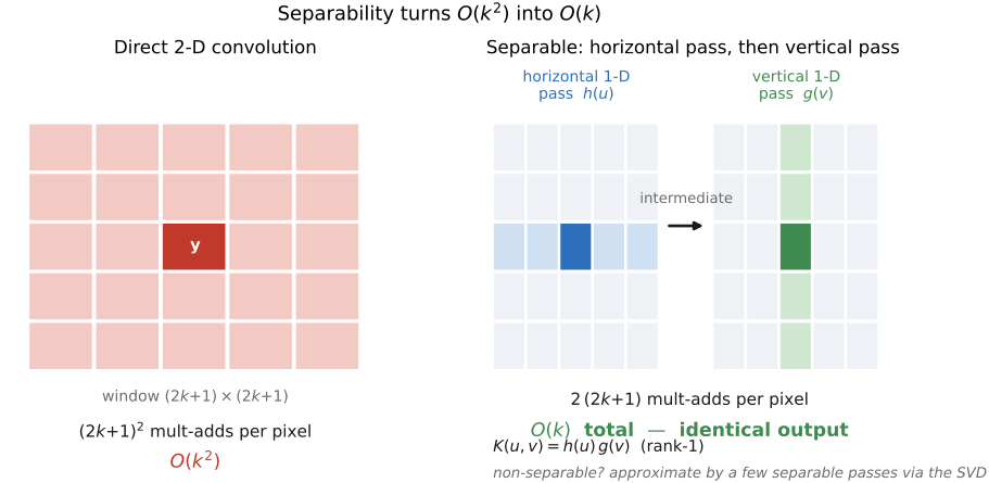
For a nonseparable kernel, its singular value decomposition gives a sum of separable terms. Retaining a few terms approximates the kernel with a corresponding error. Compare the resulting images as well as the kernel norm; see Chapter 6.2, Convolution.

The next accelerations share another form of reuse. A running sum retains what overlaps between successive windows. A prefix table retains cumulative sums for later rectangle queries. A sliding histogram retains counts so the next median need not start from a new sort. Each chooses a state that can be updated more cheaply than recomputing the answer from its definition.

29.1.3 Recursive / IIR filters: a running state, cost independent of radius🔗⧉

For a one-dimensional box, retain the sum rather than recomputing it:

Moving one pixel removes one sample and adds one. Initialize the first sum, apply the chosen boundary rule, and normalize. Horizontal and vertical passes give a two-dimensional box. Initialization still costs work; “constant time” describes the update per output, not processing an entire image in constant time.

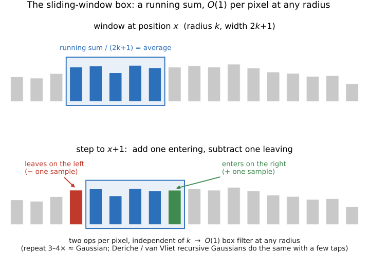
Repeating boxes produces a Gaussian-like kernel; the number and widths of the boxes determine its approximation. Recursive IIR filters use a fixed number of states and forward/backward passes to approximate Gaussian filtering more directly [@deriche-1993; @vanvliet-etal-1998]. Their per-sample arithmetic can remain fixed as the desired scale changes, but coefficient accuracy, boundary initialization, and numerical stability still matter.

Recurrences introduce dependencies along scanlines. Independent rows or columns provide parallelism, while splitting a recurrence requires more care than splitting an independent stencil. Choose accumulators from bounds on the running state and test for drift on long lines. Precision matters elsewhere too; Chapter 29.9, 8-bit and fixed-point arithmetic develops those checks.

29.1.4 Integral images / summed-area tables: any box sum in four lookups🔗⧉

Define a zero-padded prefix table on pixel boundaries:

For integer endpoints, the sum over the half-open rectangle $[x_0,x_1)\times[y_0,y_1)$ is

Divide by $(x_1-x_0)(y_1-y_0)$ for its mean. After $O(N)$ preprocessing, each rectangle query uses four table reads regardless of area. Evaluating more rectangles still costs proportionally more queries.

Crow used summed-area tables for texture filtering Crow 1984; Viola and Jones used integral images to evaluate rectangular features efficiently Viola & Jones 2001. The table stores sums over potentially the whole image. An unsigned 8-bit image with 12 million samples can accumulate to 3.06 billion, beyond signed 32-bit range. Choose a sufficiently wide type; floating-point tables can lose accuracy when subtracting large, nearby prefix sums to obtain a small rectangle.

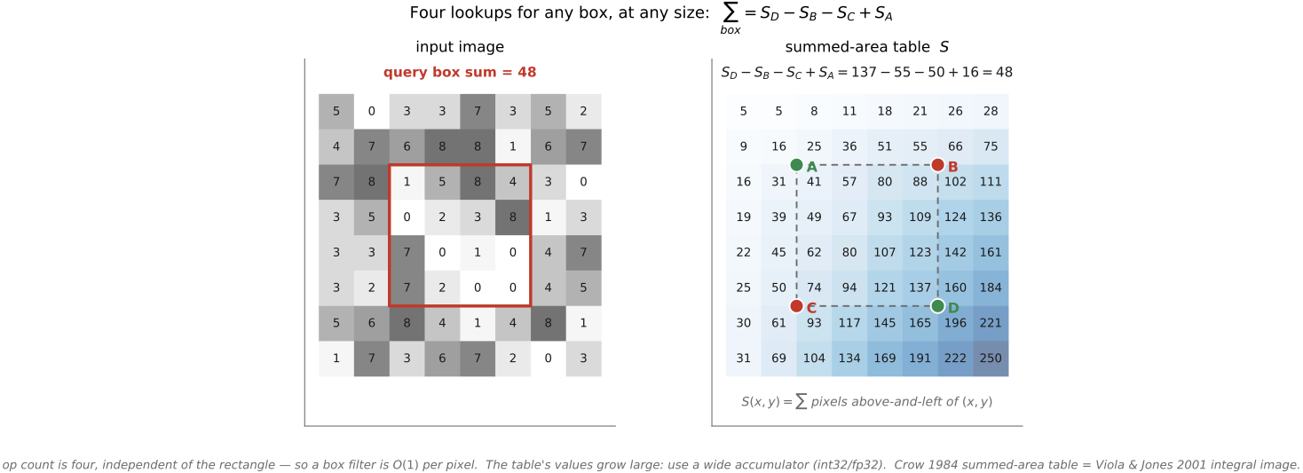
Read the four-corner formula as inclusion and exclusion. The bottom-right prefix contains the desired rectangle plus two unwanted strips. Subtract the prefixes along its top and left, then add back the top-left overlap that was removed twice. The same data structure served texture filtering in graphics and rectangle features in vision under different names. Recognizing the shared operation makes an acceleration from one problem available in another.

29.1.5 Fast median filters: a sliding histogram for a constant-time median🔗⧉

The median is nonlinear; it is not a separable convolution. Sorting each window is also unnecessary. For a bounded discrete intensity domain, maintain histograms and find the median by accumulating counts to the middle rank.

For radius-independent updates, keep a histogram of the current vertical window for every column. Moving down a row removes and adds one sample per column. Moving the horizontal window combines the entering and departing column histograms. With $B$ intensity bins, a straightforward combination and median search cost $O(B)$ per output, independent of radius, with additional storage and initialization. Adding and removing each pixel of a whole column directly would still cost $O(k)$ per horizontal step.

Weiss Weiss 2006 and Perreault and Hébert Perreault & Hébert 2007 develop efficient histogram methods. The fixed-domain assumption matters: 256 bins are practical for 8-bit values, while high-bit-depth or floating-point data require another representation or quantization. See the constant-time median paper.

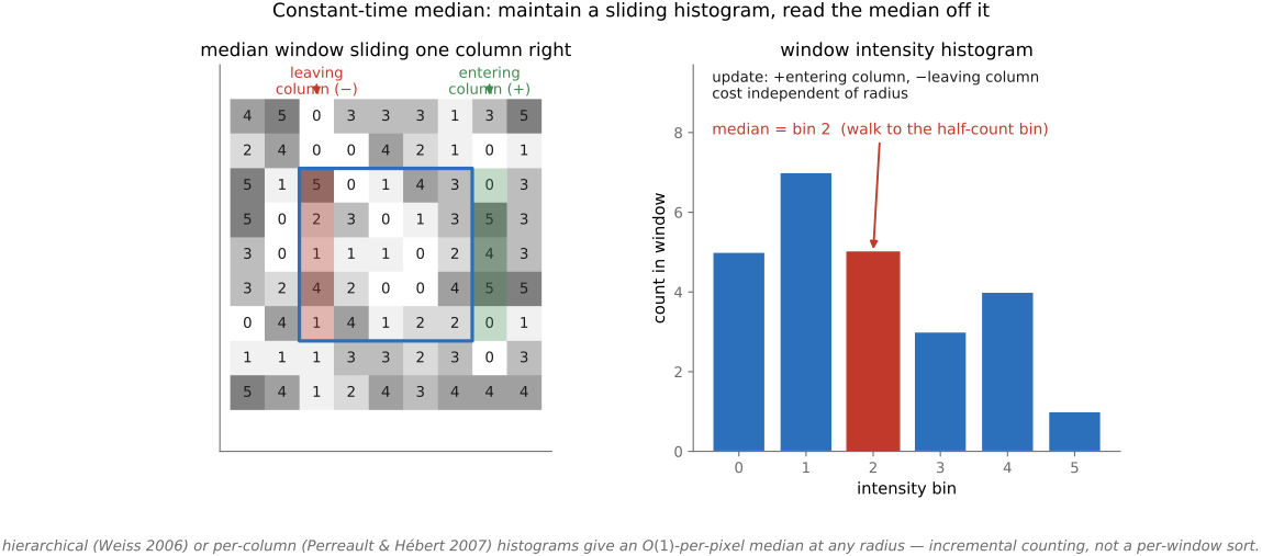
Imagine an 8-bit image and a 9×9 window. The median is the value at which the cumulative histogram first reaches 41 of the 81 samples. Moving the window one pixel right retains 72 samples, removes a column of nine, and adds another column of nine. Re-sorting all 81 values discards that overlap. Updating the histogram reuses it.

Column histograms extend the reuse in the vertical direction: advancing a column's window removes one old sample and adds one new sample. The two-dimensional window histogram is assembled from those column histograms. The cost of adding histogram arrays and finding the median depends on the number of bins, which is fixed at 256 in this example. That fixed alphabet is what permits radius-independent formulations; it is not a constant-cost guarantee for arbitrary floating-point values or unlimited precision.

29.1.6 Pyramids and multiscale: do the large-scale work on small images🔗⧉

Low-frequency work can often be done on a smaller image. Low-pass filter before reducing the resolution, compute at the appropriate scale, and reconstruct. If each level halves both dimensions, the total pixel count is

Thus a fixed amount of work per pixel per level remains $O(N)$ over the pyramid Burt & Adelson 1983 (Laplacian pyramid). This does not make every multiscale solver linear-time: iterations and work per level must also be bounded. Nor does filtering a coarse image and upsampling generally equal the original full-resolution convolution. Chapter 6.6, Pyramids and wavelets develops the sampling and reconstruction details.

29.1.7 Discretize the range to accelerate non-linear filters🔗⧉

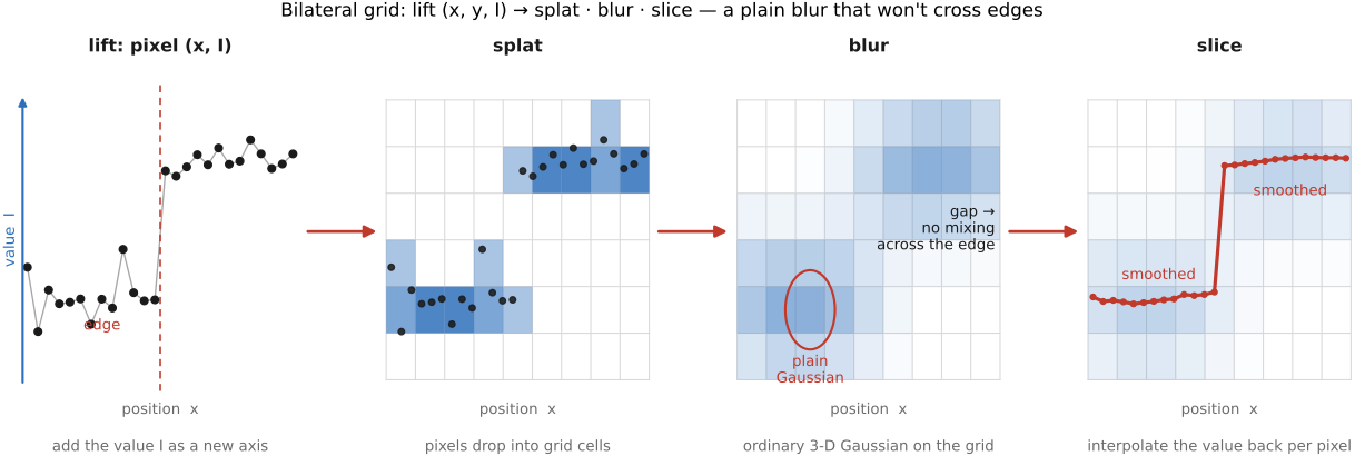
For edge-aware filters, useful structure may lie in intensity as well as position. The bilateral grid Chen et al. 2007 accumulates image values and weights on a coarse $(x,y,I)$ grid, blurs both arrays, then interpolates and divides the accumulated value by the accumulated weight. Nearby positions with very different intensities have less influence on each other, not necessarily zero influence. The splat and slice depend on the image, so the complete operator remains nonlinear even though the grid blur is linear.

Fast local Laplacian filtering Aubry et al. 2014 approximates the operator of Paris and colleagues Paris et al. 2011 by evaluating remappings at sampled reference intensities and interpolating appropriate pyramid coefficients. The number of samples controls work and approximation quality. Both methods replace repeated local computation with reusable work over a discretized range; see Chapter 10.1, Bilateral filtering and Chapter 10.4, Local Laplacian filters.

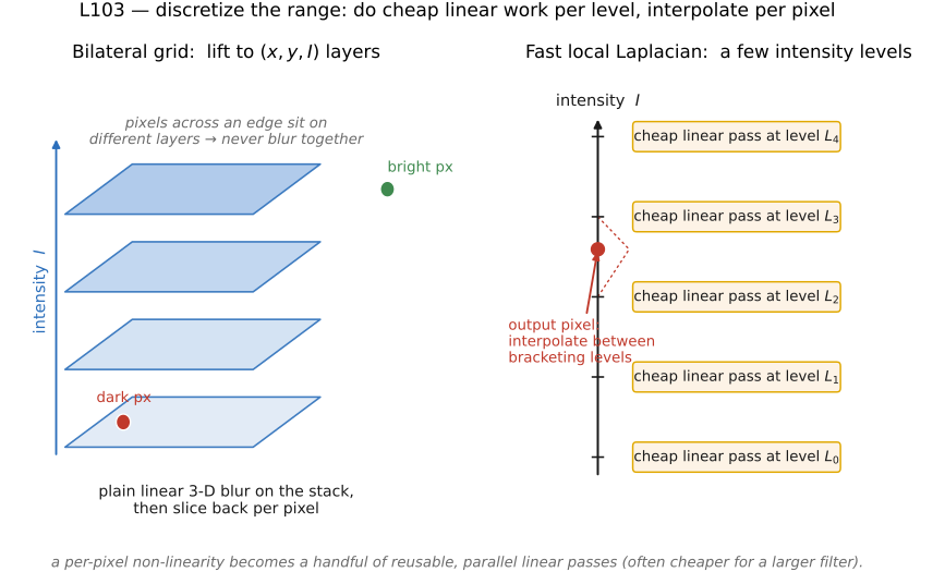
In a bilateral grid, two neighboring pixels with very different intensities are separated along the grid's intensity axis. A compact blur in that lifted space can therefore combine spatial neighbors with similar values more strongly than those across an intensity edge. The splat and slice still depend on the image, so this linear grid blur does not turn the complete filter into a linear operator. The fast local Laplacian method uses a related discretization: evaluate remapped pyramids for a set of reference intensities, then interpolate the required coefficient rather than building a new pyramid for every output location Aubry et al. 2014. In both cases, the intensity sampling trades accuracy against repeated computation.

29.1.8 Downsampling and edge-aware upsampling🔗⧉

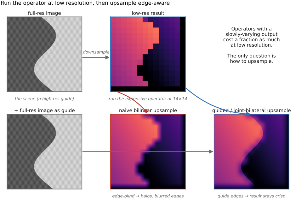
Another useful approximation computes a low-resolution field of adjustments and applies it to the full-resolution image. A global exposure or color transform is an especially simple case; spatially varying tone adjustments can often use a coarse field. The final image still retains the original high-frequency detail because the field controls a transformation rather than replacing the image.

For example, suppose an expensive operator chooses a spatially varying exposure adjustment. Reducing each input dimension by eight gives it one sixty-fourth as many pixels to inspect. The final photograph still needs work at every output pixel, but applying an exposure field is much cheaper than estimating it. That is the opportunity: spend the expensive work estimating a compact transformation, then apply it to the original samples. It is different from simply enlarging a low-resolution finished photograph, which would lose its fine detail.

Depth, mattes, and transmission can have sharp boundaries or thin structures. They are not generally smooth enough to recover by ordinary interpolation. Joint bilateral upsampling Kopf et al. 2007 (joint bilateral upsampling) uses a high-resolution guide to weight nearby coarse estimates. It can preserve boundaries that correspond to guide edges, but may transfer texture from the guide or miss a depth boundary with little color contrast. A guide cannot supply a missing thin structure merely because the upsampler is edge-aware.

In joint bilateral upsampling, take a fine output pixel and visit nearby coarse estimates. Spatial distance determines which coarse positions are relevant. The guide supplies a second weight: a coarse estimate associated with a very different guide color should have little influence, even when it is close. Normalize the surviving weights before averaging the coarse values. If the coarse result distinguishes the two sides of a silhouette and the guide locates the boundary more accurately, the estimate can change at that fine boundary instead of bleeding through it.

for each full-resolution position:
    numerator = 0
    denominator = 0
    for each nearby low-resolution estimate:
        compare its guide value with the guide at the output position
        weight = spatial_weight * guide_similarity_weight
        numerator += weight * low_resolution_estimate
        denominator += weight
    output = numerator / denominator, with a defined fallback if weight is zero

The guide contains high-resolution structure, but no new measurement of the quantity being upsampled. A painted stripe can be a strong color edge with no depth discontinuity. A foreground object can share its background's color. These examples explain both texture transfer and missed boundaries without treating edge-aware upsampling as a substitute for acquiring the missing evidence.

The guided filter He et al. 2010 fits local affine models

with regularization, then averages the models from overlapping windows. Guided upsampling estimates coefficients at low resolution and interpolates them for application to the full-resolution guide. Box-filter statistics make the fitting efficient. The model encourages agreement with guide structure; it does not guarantee artifact-free boundaries.

Bilateral guided upsampling Chen et al. 2016 (bilateral guided upsampling) represents transformations with affine models over a bilateral grid. HDRnet Gharbi et al. 2017 predicts a grid of affine coefficients from a downsampled image and slices it using a learned guide before applying the transforms at full resolution. This works well for operations represented by local color transformations. It cannot reproduce arbitrary geometric warps or synthesize missing texture solely with a pointwise affine color transform.

The same structure can be learned. Replace the hand-built low-resolution computation with a learned one and you get HDRnet (Gharbi, Chen, Barron, Hasinoff & Durand 2017) Gharbi et al. 2017: a neural network looks at a downsampled input and predicts the bilateral grid of affine coefficients; the full-resolution output is produced by slicing those coefficients and applying the resulting per-pixel affine transform. The expensive coefficient-prediction network runs at low resolution; full-resolution work computes the learned guide, performs an edge-aware trilinear slice, and applies the affine transform, as demonstrated for viewfinder enhancement on the phones evaluated in the paper. This is the pattern in its simplest form: predict coefficients at low resolution and apply them at full resolution.

The information split explains both the speed and the limitation. The coarse computation supplies adjustment values or model coefficients; the original high-resolution image supplies detail to which they are applied. In joint bilateral upsampling, a coarse estimate has less influence on a fine pixel when their guide values differ strongly, even if their positions are close. In bilateral-grid slicing, fine pixels on opposite sides of an intensity edge sample different heights of the grid. Neither requires generating the full-resolution output by ordinary interpolation of a small finished photograph. Both can fail when the guide’s distinctions do not correspond to the distinctions the output needs.

29.1.9 Choosing a method🔗⧉

Choose by workload. A separable FIR is simple for a small fixed kernel; running sums suit boxes; prefix tables suit repeated rectangle queries; recursive and multiscale methods offer approximations for wide filters. For a large nonseparable convolution, FFT methods are another option; account for padding and boundary conditions as described in Chapter 6.3, Fourier.

Benchmark setup, intermediate storage, and repeated use as well as arithmetic. Measure approximation error on the intended inputs. A lower asymptotic count helps only after its constants and memory costs are paid.