28.12 Displaying images together🔗⧉

Every chapter of this part has treated a photo collection as a problem to search, align, average, or mine. This last one treats it as a thing you make: an arrangement of images, shown together, for someone to look at. That is an older craft than the algorithms in the book: the photo album, gallery wall, contact sheet, and slideshow. The part ends there, because the point of accumulating thousands of pictures was never the pictures. It was the experience you can compose from them.

A display of many images is really three choices stacked on top of each other: which images you show (selection), where each one goes (layout), and how they sit together as a whole (color and coherence). Each has a little engineering behind it and a great deal of judgment, and the engineering is most useful precisely when it serves the judgment rather than replacing it.

28.12.1 Selection🔗⧉

You almost never show everything. A holiday is two thousand frames; the wall holds twelve. So the first act of display is selection, and it pulls in two directions at once: toward the representative (show what the collection is about, meaning the typical or strongest images) and toward the diverse (show its range, so you do not print twelve near-identical sunsets). The auto-curation machinery of Chapter 28.3, Auto curation gives you the raw material, such as quality scores, near-duplicate clustering, and face and event detection, but the choice of how much representativeness to trade for diversity is a matter of intent: a memorial wall wants the typical, a portfolio wants the range. In practice the good workflow is a human in the loop: let the machine propose a diverse, high-quality shortlist, then choose by hand, because the thing you are optimizing (what this set should feel like) is not something a score knows.

(author: Frédo's own selection practice and how he narrows a shoot to a set; placeholder for his themes and rules of thumb.)

28.12.2 Layout🔗⧉

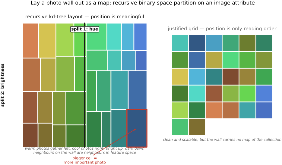
With the images chosen, layout decides where each one lands in 2-D, and the main choice is whether position carries meaning. The simplest layout is the justified grid (the Flickr/Google-Photos row-packed wall): pack images into rows of equal height, fill the width, and position says nothing but reading order. It is clean and it scales, and for a chronological stream it is exactly right.

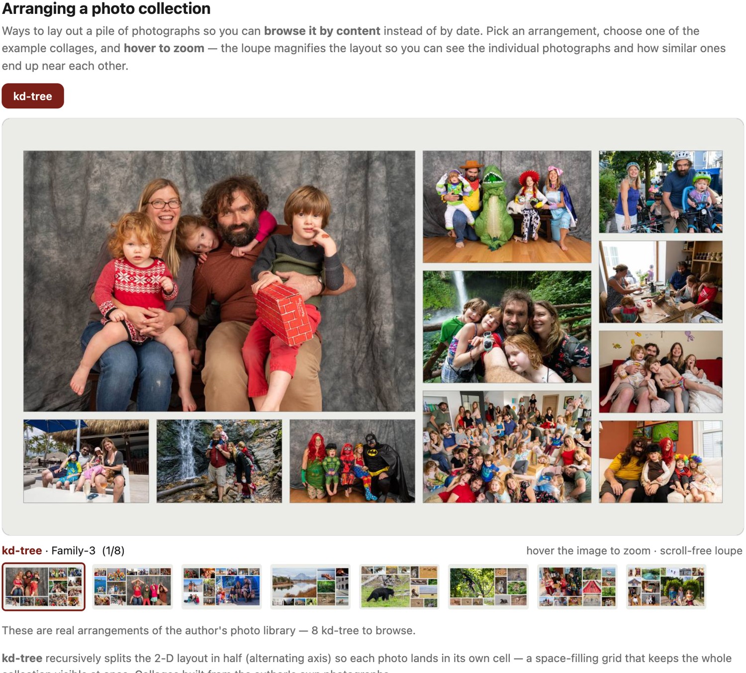
But you can make the wall itself a map. The author's approach is a recursive kd-tree layout: split the canvas with a line, split the photo set by an attribute (hue, brightness, time, or a similarity coordinate) at the same fraction, and recurse, producing a binary space partition that groups images along the selected attributes. A two-dimensional arrangement cannot preserve every neighborhood in a high-dimensional descriptor space. Reds drift to one corner and blues to another; mornings cluster apart from nights; a region of the wall becomes a region of the collection. Because the partition is binary and area-proportional, it packs tightly with no wasted space and gives every image a rectangle whose size you can tie to its importance (a favorite gets a bigger cell). (ref: author, see …) The same idea, that 2-D position can encode similarity, drives the treemap (Shneiderman's area-proportional nested rectangles, here keyed to photo attributes) and force-directed packings; the kd-tree is the version that stays a clean, rectangular, recursively-balanced wall.

Self-organizing maps: a learned map of a collection🔗⧉

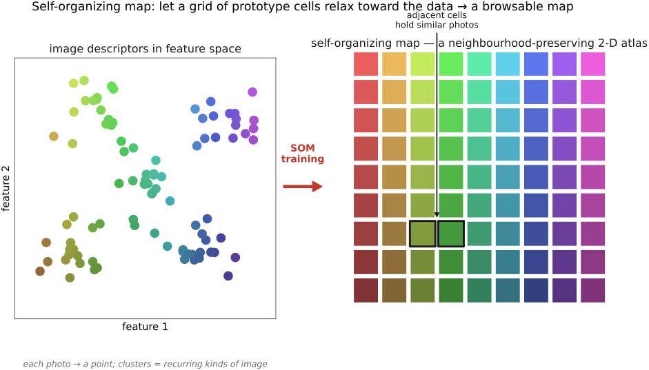
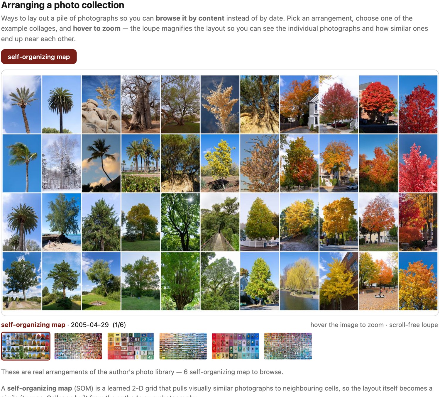
The kd-tree imposes a chosen axis on the wall; a self-organizing map (Kohonen) learns one. A SOM is a grid of cells, each holding a prototype in feature space; you present the collection's image descriptors one by one, and each pulls its nearest cell and nearby cells toward it. The grid relaxes into a neighborhood-preserving 2-D embedding of the collection: visually similar images end up in adjacent cells, and the whole map becomes a smooth atlas you can scan, with the clusters of your photographic life laid out as territories. It is the classic "map of a photo collection," and it captures the same intuition as the kd-tree (spatial proximity = similarity) but from the data's own structure rather than a hand-picked attribute, with a separate assignment problem if every photograph must occupy exactly one cell. A standard SOM grid can itself be rectangular; multiple images may map to one prototype and other cells may be unused.

Photomosaics: one picture made of many🔗⧉

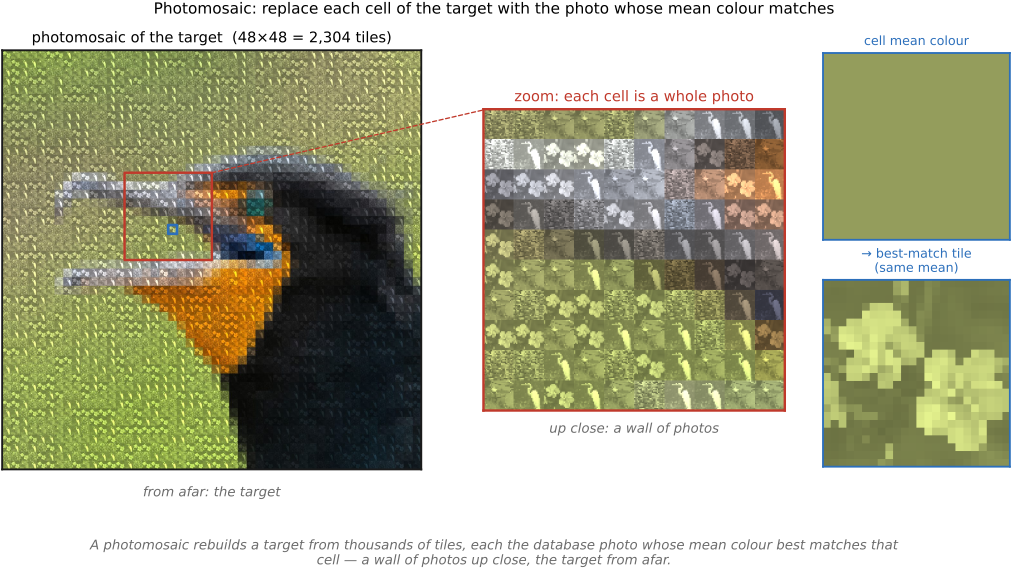
The most playful way to show many images together is to make them be another image. A photomosaic (popularized by Robert Silvers) renders a target picture as a grid of tiles, each tile a photograph from the collection chosen so its average color (and, in the better versions, its coarse structure) matches the target patch it covers. Step back and you see the target; step close and you see a thousand individual photographs, each intact. It is selection-and-layout fused into one: the target dictates both which images appear (those whose colors are needed) and where each goes (the patch it matches), and the collection supplies the palette. It is a gimmick, but a revealing one: it makes literal the idea that a collection can be a medium, not just a set.

28.12.3 Color and coherence🔗⧉

A wall of images either hangs together or it jangles, and the difference is usually color. Photographs shot across years, cameras, and lights arrive with mismatched white balance, exposure, and palette; hung naïvely they fight. So the last act of display is a gentle normalization (bring exposures into a common range, neutralize wildly different casts, perhaps nudge the set toward a shared palette) and an ordering that lets color flow rather than clash (a gradient of hue or tone across the wall, warm to cool, light to dark). This is the same perceptual budget the rest of the book spends on single images (Chapter 4.1, Color space 101, tone mapping), now spent on the relationships between images: not "is this photo right?" but "does this photo sit well next to that one?" The goal is coherence while preserving each image's character: the set should feel composed, while each picture stays itself.

28.12.4 Themes🔗⧉

(author: Frédo's own thematic collections: the recurring subjects, the long-running series, the personal taxonomies by which he groups and re-groups his photographs over the years. Placeholder for the author's themes, in his voice; this is the most personal section of the most personal chapter.)

The thread through all of it is that a collection is not finished when it is captured, or even when it is curated: it is finished when it is arranged, for someone, into something to look at. The algorithms in this part can find the photographs, align them, average them, and search them; what they cannot do is decide what the wall should mean. That is the last, human step, and the right place to end a part about many images: with the oldest question photography asks, not how to take the picture, but what to do with all of them once you have.