28.8 Pix 2 GPS🔗⧉

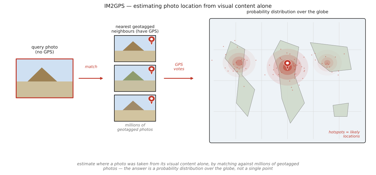
IM2GPS estimates where a photo was taken from nothing but the pixels and a giant geotagged collection. No EXIF GPS, no named landmark, no map: describe the query by its visual content, retrieve the photographs that look most like it from a database of millions of geotagged images, and let their coordinates vote on where the query was shot. The planet itself becomes the model. The key design choice is to return a distribution over locations rather than a single coordinate: a nondescript field or beach stays geographically vague, while distinctive architecture, vegetation, or signage pins the location tightly. This is the geolocation sibling of Chapter 21.3, Inpainting Using Millions of Photographs (Hays & Efros 2008, "IM2GPS") Hays & Efros 2008 (IM2GPS), and it makes the same bet as the rest of the part: that at sufficient scale, the collection is the prior.

28.8.1 Geolocation as retrieval over a geotagged corpus🔗⧉

The whole method is Chapter 28.2, Retrieval pointed at a corpus that happens to carry coordinates. Describe the query image $I$ with the same kind of global, scene-level descriptors that classic content-based retrieval uses: a mix of color histograms, texture statistics, and a coarse scene/layout descriptor (the GIST-style "gist of a scene" that captures whether you are looking at a coastline, a street, a forest, a mountain). Then find the query's nearest visual neighbors among millions of geotagged Flickr photos. Nothing in this step knows anything about geography; it only knows what the query looks like. The geography enters entirely through the neighbors' attached GPS tags, which become the evidence for where the query was taken.

That re-framing is the clever part. There is no map in the original system, no per-place classifier, no list of landmarks to match against. The database's empirical "what places look like" (accumulated, for free, from millions of strangers tagging their holiday snapshots with locations) does all the work. This is exactly the wager of Chapter 21.3, Inpainting Using Millions of Photographs: scale substitutes for a learned model. A large collection improves the chance of finding informative examples. It does not ensure coverage of an arbitrary location, and visually similar scenes can occur on different continents. Popular tourist sites and geotagging errors also shape the evidence. The descriptors and the fast nearest-neighbor search are the engine; the coordinates are just metadata that rides along.

The visual features do some things well and not others. They are good at scene type and texture, such as Mediterranean stucco versus Alpine timber, desert scrub versus tropical canopy, or the color cast of a particular sky, and at coarse layout. They are not, in this classic form, recognizing a specific building by its facade (that is the landmark-recognition problem, which leans on the local-feature, spatial-verification side of Chapter 28.2, Retrieval). IM2GPS deliberately works at the level of scene appearance, which is why it generalizes to anonymous places that no landmark recognizer would ever have cataloged.

28.8.2 The answer is a distribution🔗⧉

Once you have the query's nearest neighbors, you do not pick the single best match and copy its coordinate; that would throw away the most useful thing the method knows, which is how confident to be. Instead, aggregate the retrieved neighbors' coordinates into a probability distribution over the globe: a kernel (Parzen) density estimate that places a soft bump at each neighbor's location and sums them, so the posterior is

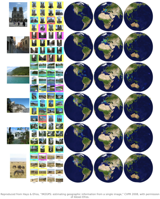
a schematic weighted sum of kernels $K$ centered on the geotags of the visual neighbors $\text{NN}(I)$. On the globe, use spherical distances and a properly normalized spherical kernel rather than ordinary latitude-longitude subtraction: longitude wraps and its physical scale changes with latitude. Where many similar-looking photos cluster geographically, the bumps pile up into a sharp peak; where the neighbors scatter across continents, the mass smears out (Figure 28.8.1⛶ fullscreen). The map, not a pin, is the deliverable.

The spread is the point: uncertainty is the result. A photo of a generic sandy beach is consistent with every warm coastline on Earth, so the truthful output is a diffuse band across the tropics and Mediterranean, and reporting that diffuseness is more useful than confidently guessing one wrong beach. A photo carrying distinctive cues (a particular style of architecture, a writing system on a shop sign, an unmistakable vegetation or terrain) collapses the mass onto a small region. The shape exposes the estimate’s alternatives, but a narrow peak is not proof of accuracy. Biased retrieval can produce confident errors; assess calibration on held-out locations and near-duplicate-free data. This is the same humility that the rest of the book prizes: a method that reports its own confidence beats one that always answers with false precision.

28.8.3 Mapping the collection itself🔗⧉

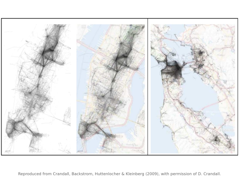
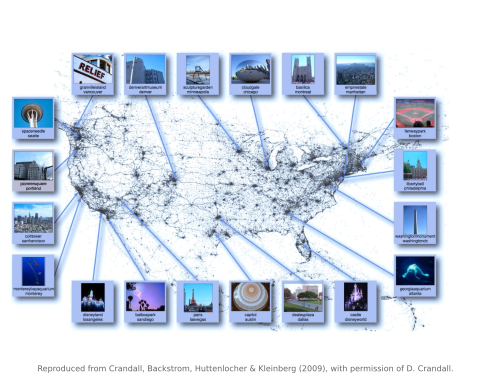
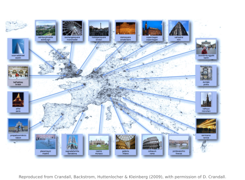
IM2GPS reads a coordinate out of the geotagged crowd; the complementary question is what the crowd's coordinates, taken together, reveal about the planet. Crandall and colleagues (2009) took the GPS tags of millions of Flickr photos and asked simply where do people point cameras? They clustered the geotags to surface the world's most-photographed places, then used visual and textual features to label and connect them. The same data-as-prior creed, aimed not at one query but at the structure of the whole collection: the photographs' locations are themselves a map of human attention.

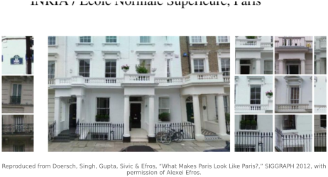
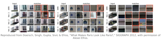
A complementary question is not just where people photograph but what makes one place look like itself: the visual signature that distinguishes one city from another. Doersch and colleagues (2012), in "What Makes Paris Look Like Paris?", mine a giant geotagged collection for mid-level discriminative patches: image fragments (a style of balcony railing, a street sign, a particular window or lamp-post) that recur in one city's photographs and almost nowhere else. It is the same data-as-prior creed turned toward distinctiveness: the collection is searched not for the typical but for the geographically characteristic, the elements a place-recognition system could key on.

28.8.4 The learned successors🔗⧉

The classic IM2GPS recipe is explicit retrieval: hand-built descriptors, a nearest-neighbor search, a kernel estimate over the neighbors' tags. The deep era keeps the task and the distribution-over-the-globe output but swaps the mechanism. PlaNet (Weyand, Kostrikov & Philbin 2016) Weyand et al. 2016 (PlaNet) reframes geolocation as classification: partition the surface of the Earth into a few thousand discrete geo-cells (smaller cells where photos are dense, larger where they are sparse), and train a deep network to classify a photo directly into a cell. The network learns the planet's appearance end-to-end from the geotagged corpus rather than relying on hand-designed color and texture features, and its softmax assigns probability mass to cells, which must be distinguished from probability density when cells have different areas: the same distributional output as IM2GPS, now produced by learned weights instead of an explicit neighbor search.

The two approaches are the geolocation instance of a pattern that recurs across this book: data-as-prior (retrieve a real coordinate from real photographs) versus weights-as-prior (bake the planet's appearance into a trained network). They share IM2GPS's founding insight (that location is recoverable from visual content and is best reported as a distribution) and they share its dependence on a massive geotagged collection. What changed is only the operator: a hand-built descriptor and a nearest-neighbor vote gave way to a learned classifier (Chapter 7.3, Deep learning). The problem Hays and Efros posed is intact; the engine under it was neuralized, exactly as it was for the embeddings of Chapter 28.2, Retrieval and for so much else in this part.