24.4 Intrinsic images with time lapse🔗⧉

Bolt a camera to a windowsill and let it shoot one frame every few minutes from dawn to dusk. Over the day you collect hundreds of pictures of the same scene: the same bricks, the same lawn, the same parked car, yet no two frames look alike. What changes is not the scene but the light: the sun arcs overhead, shadows of the eaves and the railing sweep slowly across the wall, a bright patch crawls along the ground and is gone an hour later. The bricks were always that shade of red; the lawn was always that green. The paint never moved. Only the lighting did.

That single fact is the lever. An image is, to a first approximation, the product of two things: what a surface is made of and how it is lit. The first is its reflectance (or albedo): the fraction of light each point sends back, a property of the surface itself, fixed for the day. The second is its shading: how much light actually reaches that point, which depends on the sun's position, on shadows, on the whole geometry of illumination. Pulling these two apart (recovering the paint from the light) is the classic intrinsic-images problem Barrow & Tenenbaum 1978, and from a single photograph it is hopeless: a dark patch could equally be dark paint or a cast shadow, and infinitely many reflectance/shading pairs reproduce the very same image (this is the prior-not-optional ambiguity, L7.8show, met head-on in Chapter 24.1, Illumination related effects in a single image). A time-lapse stack provides new evidence: reflectance stays fixed while illumination changes. But constant shading also stays fixed. Separating it from reflectance still requires an assumption about the illumination, even with hundreds of frames. This is the L13.1show idea once more, on a new axis.

The chapter is short because it reduces to a single, clean estimator, due to Weiss 2001: work in the log domain, take the median over time of the log-gradients, to estimate the reflectance gradient field; reconstruct with a Poisson solve, then divide each frame by the estimated reflectance to obtain its shading. The estimator is simple, but its assumptions determine which shadows it removes.

24.4.1 The split, and why one image can't do it🔗⧉

Write the model down. At pixel $(x,y)$ in the frame captured at time $t$, the observed image is the product of a time-invariant reflectance and a time-varying shading,

where $R$ is the surface albedo, the what-it's-made-of, fixed across the whole sequence, and $S(x,y,t)$ is the how-it's-lit, sliding as the sun moves and shadows sweep through. (This is the same reflectance×shading factorization behind lightness constancy, developed in Chapter 3.3, Visual processing; here we exploit it across frames rather than within one.) Intrinsic-image decomposition is the task of recovering the two factors $R$ and $S$ from the observed $I$.

From one frame this is fundamentally under-determined. There is one equation and two unknowns at every pixel, $I = R\cdot S$, so for any observed $I$ there are infinitely many factorizations: scale $R$ up by any amount and $S$ down by the same amount, and the product is unchanged. Is that dark region on the wall dark brick or the shadow of the railing? The pixel alone cannot say. Single-image methods break the tie only by importing an assumption about how reflectance and shading differ: the Retinex prior, for instance, declares that large gradients are reflectance edges (a sharp boundary between two paints) while gentle, smooth gradients are shading (light falling off softly), then thresholds the gradient field on that basis and integrates. That works, but it is a hand-built prior, and it is not optional: remove it and the problem has no answer. This is the single-image, ill-posed version of the story, and it is the subject of Chapter 24.1, Illumination related effects in a single image (L7.8show, the prior is not optional).

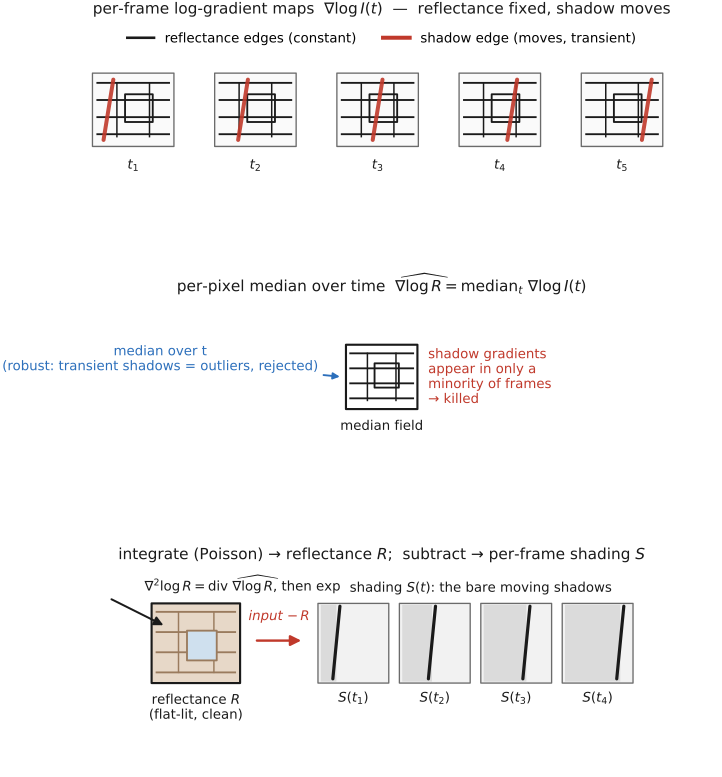
The time-lapse stack supplies evidence that one frame lacked. Fix the camera so the scene registers pixel-for-pixel, and assume its reflectance remains constant. Temporal variation can then be assigned to illumination, but a spatially varying, time-independent factor $h(x,y)>0$ remains ambiguous: $R'=Rh$ and $S'=S/h$ reproduce every frame. A stationary shadow is a concrete example. To estimate reflectance, Weiss assumes sparse, approximately zero-centered responses when derivative filters are applied to log illumination. The extra frames make that prior more useful; they do not replace it (Figure 24.4.1⛶ fullscreen).

24.4.2 Weiss 2001: the median of log-gradients🔗⧉

Yair Weiss (2001), in Deriving Intrinsic Images from Image Sequences, turns the reading rule into a one-line estimator. Two moves do all the work: go to the log domain, and take the median over time.

Go to log. The model is multiplicative, and multiplicative quantities are awkward, but a logarithm turns a product into a sum. Taking logs,

so the observed log-image is the sum of a constant log-reflectance and a time-varying log-shading. This is the same encoding lesson that recurs throughout the book: radiometry is done in linear light, and ratios become differences in log (L2.6show/L4.6show). Because gradients are linear, the spatial gradient of the log-image is likewise a sum,

where $\nabla$ is the spatial gradient (the same per-pixel $x$- and $y$-difference field from Chapter 10.8, Poisson image editing). The first term, the reflectance gradient, is the same in every frame. The second, the shading gradient, moves: a shadow edge produces a large gradient where it currently sits, and nothing where it is not.

Take the median over time. Now look at one pixel across the whole stack and ask what its log-gradient does over time. The reflectance contribution $\nabla\log R$ is a fixed vector present in every frame: at a true brick-to-mortar edge, every frame sees that edge. The shading contribution $\nabla\log S(t)$ is transient: a moving shadow edge passes over this pixel in only a minority of frames, lighting up the gradient there for a little while and then leaving. In the language of the averaging chapter, the persistent reflectance gradient is the signal and the passing shadow edges are outliers, and the right tool against outliers is not the mean (which a single hard shadow edge would drag) but the median, which resists a minority of arbitrarily large outliers. It does not generally remain numerically unchanged when some samples change. For horizontal and vertical derivatives, estimate each component separately by its temporal median:

This is accurate when each component of $\nabla\log S$ has temporal median near zero. A shadow boundary that passes briefly can then be rejected. A persistent illumination gradient is instead absorbed into the reflectance estimate. It is a robust estimator in one line, using a hand-built illumination prior rather than a trained model (Figure 24.4.2⛶ fullscreen). (Like any robust combine across a stack, this is the same reject-or-average instinct as the median in the denoising chapter, now applied across frames to gradients rather than to pixel values.)

Reconstruct L10.4show. The median gives us a gradient field for log-reflectance, not the log-reflectance image itself, so the final step is to integrate that field back into an image. This is exactly the gradient-domain reconstruction of Chapter 10.8, Poisson image editing: find the image whose gradients best match the prescribed field, which is the Poisson equation

solved by the same sparse least-squares machinery: conjugate gradient, multigrid, or a fast Fourier transform (FFT) solve. (The median field is generally not the gradient of any single image: the moving shadows leave it non-conservative, so this is genuinely the least-squares projection, not an exact integration; that is precisely why a Poisson solve is the right and necessary tool, per the conservative-field discussion in Chapter 10.8, Poisson image editing.) The solve needs boundary conditions and a fixed mean or reference value to remove its additive ambiguity. Exponentiating gives an estimated reflectance image, up to a multiplicative scale. Persistent shadows and departures from the model may remain. And once $R$ is known, the per-frame shading falls out by subtraction, one image per frame,

leaving a shading sequence relative to the estimated reflectance. Errors in that estimate appear in every recovered shading frame.

Use registered, linear, unclipped images with consistent color processing. A spatially uniform exposure multiplier disappears under spatial log differentiation, but nonlinear tone mapping does not. Mask moving objects, saturated samples, and unreliable near-black values; a small positive floor avoids taking the log of zero but does not recover missing signal. For RGB, apply the model channelwise only where that approximation is appropriate.

for each registered frame t:
    valid[t] = reliable, unclipped, stationary pixels
    logI[t] = log(max(linearI[t], epsilon))
    gx[t], gy[t] = spatial_derivatives(logI[t])
gxR = temporal_median(gx, valid derivative samples)
gyR = temporal_median(gy, valid derivative samples)
logR = least_squares_gradient_reconstruction(gxR, gyR,
                                              boundary_conditions, fixed_mean)
R = exp(logR)
S[t] = linearI[t] / R

The log transform, robust estimation, and gradient-domain reconstruction each have a distinct role. Temporal variation supplies repeated observations, while the sparse illumination-gradient prior selects their common reflectance explanation.

24.4.3 Passive and controlled illumination🔗⧉

Time-lapse decomposition is a passive form of multiple-image capture. As with HDR exposures, focal stacks, and spectral measurements, the camera records variation along an additional axis L13.1show. Here the axis is time under changing illumination. The camera does not need to control the sun, but it must wait for useful changes while the scene remains sufficiently stable.

Part 35, Computational illumination instead includes techniques that deliberately control the light: flash/no-flash pairs, multi-flash imaging, photometric stereo, and structured light. These techniques use different forward models and recover different quantities, but they share the strategy of making illumination changes informative. Controlled capture can arrange observations that a passive time lapse may never provide, such as moving a shadow that otherwise stays fixed throughout the sequence.