22.9 Autofocus🔗⧉

The ideal focused lens has one sharp conjugate object plane; real aberrations can curve or split the best-focus surface. Everything closer or farther blurs, gently at first and then badly, into the circles of confusion that FUNDAMENTALS made precise. The previous chapter showed that moving the focus is mechanically almost trivial. The hard part is the decision. Given the blurry image the sensor sees right now, is the subject in front of the focal plane or behind it, and by how much? A camera that cannot answer the second question can still focus. It just has to guess and check, nudging the lens and watching whether the picture got sharper or worse. A camera that can answer it focuses in a single confident move. This chapter moves from the first kind to the second, and then reuses the machinery, since defocus carries depth, to measure the scene's 3D shape.

22.9.1 Contrast-detection AF🔗⧉

The first algorithm is the most direct, and it needs no special hardware at all, just the imaging sensor the camera already has. The premise is a single observation about defocus: a sharp image contains more high-frequency energy than a blurred one. Blur is a low-pass operation; it smears edges, attenuates fine detail, and flattens the local contrast. So if you measure how much high-frequency content the image has and maximize it over lens position, a suitable metric usually peaks near the desired focus, provided the region contains usable detail and noise or processing does not dominate. This is contrast-detection autofocus (CDAF).

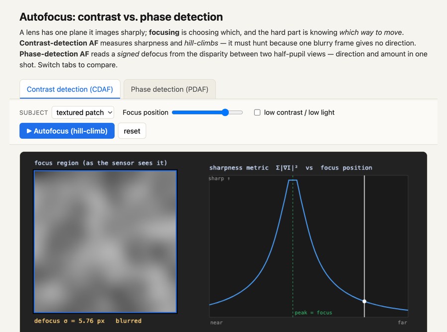
Concretely, the camera computes a contrast metric over the focus region: a sum of squared image gradients, or the energy passing a high-pass filter, or the variance of the local Laplacian. Any of these rises as the image sharpens and falls as it blurs, often tracing out a dominant peak, though texture, multiple depths, noise, or defocus transfer-function lobes can produce competing peaks as the lens sweeps through focus (Figure 22.9.1⛶ fullscreen). Finding focus is then gradient ascent on the sharpness curve: climb until the metric stops increasing, and you are at the peak.

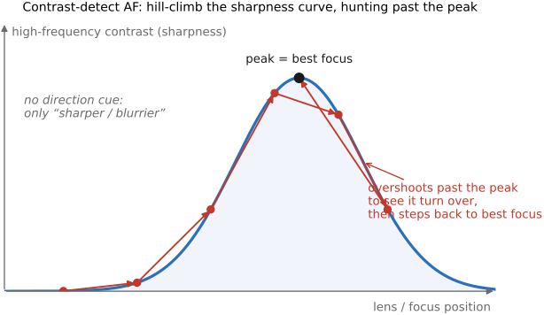
Contrast detection's strength is that it evaluates the recorded image directly: it reads the very sensor that will take the picture, so it avoids a separate AF optical-path mismatch. Metric choice, subject motion, noise, lens motion, and aperture-dependent focus shift can still affect accuracy. Its main weakness follows from the use of gradient ascent. A single measurement of the metric tells you the image's sharpness but not the slope of the hill. From one blurry frame the camera cannot tell whether focus lies nearer or farther: both directions look equally blurry. So it must hunt: nudge the lens one way, measure again, and infer the direction from whether the metric rose or fell, possibly reversing if it guessed wrong. This trial-and-error is visible as the lens racking back and forth before settling, it is slow, and it fails outright in low contrast or low light, where the hill is so flat that sensor noise swamps the metric and the peak is undetectable. Contrast AF is accurate but blind to direction. The next method fills that gap.

22.9.2 Phase-detection AF (the split-pupil / stereo trick)🔗⧉

Suppose that instead of one view of the scene you had two, taken from two different parts of the lens's aperture. Then you would have a stereo pair, and stereo gives you not just that the subject is out of focus but which way and how far, in a single shot. This is the idea behind phase-detection autofocus (PDAF).

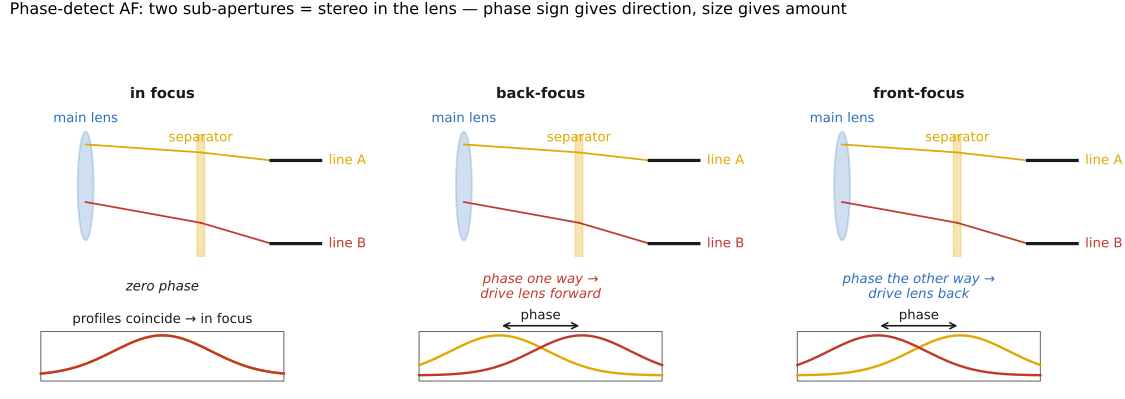
The geometry is straightforward. Light from a single subject point fills the whole exit pupil of the lens and converges toward the conjugate image point. If the sensor sits exactly at that convergence point, all the rays (from the left of the pupil, the right of the pupil, everywhere) pile onto one spot: in focus. But if the sensor is in front of the convergence point, the cone has not finished closing, and rays from the left half of the pupil land to one side while rays from the right half land to the other; the two half-pupil images are separated. If the sensor is behind the convergence point, the cone has crossed over, and the two half-pupil images separate the other way. The separation between the two half-pupil views is therefore a signed quantity: its sign tells you the direction of defocus (front or back), and its magnitude tells you how far out of focus you are.

A dedicated PDAF module makes those two views explicit. After the main lens, a small separator (secondary) lens, really a pair of tiny lenslets behind a mask, re-images the left and right halves of the exit pupil onto two separate line sensors. When the main lens is focused, the two line patterns line up. When it is defocused, the two patterns slide apart by an offset proportional to the defocus, with a sign set by the defocus direction (Figure 22.9.2⛶ fullscreen). The camera correlates the two line signals to read off that lateral offset in one measurement, and from the offset it estimates the direction and size of a focus correction using a calibrated lens model. A confirmation or tracking update may still be needed; weak or repetitive texture can make the correlation ambiguous. This is why phase detection is faster than contrast detection.

PDAF uses a stereo-like measurement inside one lens. The effective baseline is the separation between the pupil regions' centroids, not the physical separation between neighboring sensor photodiodes. Unlike ordinary parallel-camera stereo, the disparity is zero at the current focus distance $Z_f$, not at infinity. In a thin-lens model with sensor distance $v$ and effective pupil baseline $B$, one sign convention gives

Here $d$ is a signed separation on the sensor and $Z$ is object distance; divide by pixel pitch for disparity in pixels. Swapping the half-pupil labels reverses the sign. Compound lenses and separator optics require calibration of the scale, zero, and focus-motor response. This signed inverse-depth difference is why PDAF can suggest which way to move from a single exposure.

The classic implementation lives in the SLR. The main reflex mirror is partly transparent; behind it a small sub-mirror angles a fraction of the light downward to a dedicated PDAF module in the floor of the mirror box, with its separator lenses and line-sensor arrays (often arranged in a cross or a grid of points across the frame). This gives the fast, single-shot focus that made action and sports photography practical with autofocus. Its drawback is structural: the AF sensor is on a separate optical path from the imaging sensor, so any mechanical discrepancy between the two shows up as front- or back-focus error that must be calibrated out per body and per lens. Move the focusing function onto the imaging sensor itself and that separate-path mismatch disappears, though pupil and lens-response calibration remain, which is the next step.

22.9.3 On-sensor PDAF and dual-pixel AF🔗⧉

Phase detection's payoff (signed, single-shot focus) is too good to leave stranded on a separate module, especially once cameras went mirrorless and lost the sub-mirror entirely. The fix is to capture the two pupil halves on the main imaging sensor, so the same pixels that take the picture also report phase. There are two ways to do it.

The first is masked (phase-detect) pixels. Scatter a sparse set of special pixels across the imaging array, each with half of its light-collecting area masked off, some masked on the left, some on the right. A left-masked pixel sees only light coming from the right half of the pupil, and vice versa; pairing nearby left- and right-masked pixels recovers the two half-pupil views directly on the recording sensor. This brings PDAF to mirrorless and live-view shooting without a separate AF module and its optical-path alignment. The cost is that masked pixels are partially blind (they collect less light and must be interpolated over in the final image, like defective pixels), so they are kept sparse, which limits how dense and low-light-capable this flavor of on-sensor PDAF can be.

The second way wastes no light at all: dual-pixel autofocus. Instead of masking, split every photosite into two side-by-side half-photodiodes sharing one microlens (Figure 22.9.4⛶ fullscreen). The microlens, the same per-pixel microlens stack introduced in FUNDAMENTALS, focuses the incoming cone so that the two half-diodes respond preferentially to opposite pupil regions; the left/right correspondence depends on the ray geometry and labeling convention. Each pixel is therefore its own miniature phase-detect pair, and the architecture can provide dense phase samples; the active AF area and readout selection depend on the camera and mode. Compare the left-diode image to the right-diode image across the frame and you get a dense disparity signal (phase detection at every point), which is why dual-pixel AF is fast and tracks well across the whole frame. For the final photograph the two halves are simply summed into a normal pixel value, so no light and no resolution is thrown away.

That same dense disparity is also a depth signal: the two half-pixels form a stereo pair with an effective baseline set by the pupil, often on a millimeter scale in phone cameras, enough to read a coarse per-pixel depth. Google's Portrait Mode (Wadhwa et al. 2018) turns it into synthetic bokeh: combine the noisy dual-pixel depth map with a learned person-segmentation mask, then apply a depth-dependent blur so the subject stays sharp while the background melts away. A single small phone camera fakes the shallow depth of field of a fast portrait lens, from autofocus hardware that also provides a useful depth cue, at a cost in readout, calibration, and computation (the depth-from-defocus story the chapter closes on, pushed all the way to a product).

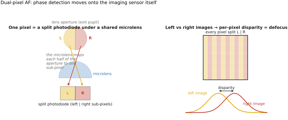
The disparity these dense methods produce is both a focus signal and a low-resolution depth signal. Because the baseline is just the small split across a single lens's pupil, the disparities are tiny and the depth map is coarse and noisy, far weaker than a wide-baseline two-camera rig. But it is real depth, captured by the main sensor in one exposure, and it is exactly what feeds portrait-mode background blur and small post-capture refocus on phones (forward-ref to the computational-DoF treatment in Depth of field and the light-field part). The same disparity that aims the lens also begins to measure the scene, which brings us to the explicitly computational siblings of autofocus.

22.9.4 Depth from focus / defocus, and learned subject AF🔗⧉

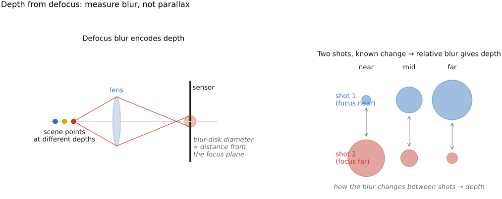
Autofocus reads defocus to remove it. If you use defocus to measure the scene, the same physics becomes a depth sensor. Two classic recipes do this.

Depth from focus (DfF) sweeps the lens through its whole focus range while capturing a stack of images, then asks, for each pixel independently, at which focus setting was it sharpest, using the very contrast metric from contrast AF, evaluated per pixel. The focus position of each pixel's sharpness peak maps directly to that pixel's depth, since each focus setting corresponds to one in-focus distance. It needs many exposures and a calibrated mapping from focus setting to distance, though it can avoid explicitly fitting a parametric blur kernel. Breathing, motion, and depth boundaries complicate correspondence across the stack. This is precisely the machinery behind focus stacking, which keeps the sharpest pixel from each slice to build an all-in-focus image rather than a depth map. The full treatment lives in Depth of field.

Depth from defocus (DfD) is the simpler alternative: rather than sweeping the entire range, take just two or a few images at different focus or aperture settings and infer, per pixel, the blur radius of the defocus disk. The geometry from FUNDAMENTALS' depth-of-field section ties that blur radius to distance-from-focus and aperture, so estimating the blur recovers the depth, from a handful of shots instead of a full stack (Figure 22.9.5⛶ fullscreen). The foundational work is Pentland's 1987 method and Subbarao's contemporaneous analysis; both estimate the local point-spread function (PSF) and solve for the depth that explains it. That defocus PSF is also the bridge to deconvolution: if you know the blur, you can both read depth from it and undo it, tying DfD to the deblurring and aberration-correction machinery in Aberrations correction.

There is a third use of the same physics, halfway between measuring depth and aiming the lens: depth from defocus as autofocus, the trick behind Panasonic's DFD (Depth From Defocus) system. Rather than build a depth map at all, it uses defocus to drive focus. The camera carries a stored model of how a given lens's blur PSF changes with focus, captures two frames at slightly different focus settings, and compares them against that model to infer not just that the image is defocused but the direction and amount of the defocus, a PDAF-like, near-single-step cue extracted from an ordinary contrast-detect sensor with no phase pixels on the array. In effect it recovers phase detection's signed error from defocus comparison alone. It rides on top of CDAF (confirming focus at the sharpness peak) and can reduce the search needed by ordinary contrast AF. Continuous-video behavior still depends on motion, texture, lens drive, and focus confirmation; it is not a guarantee of hunting-free tracking. Some newer Panasonic systems combine DFD with on-sensor phase detection. Its weakness is the dependence on a per-lens blur profile (so it works only with characterized lenses) and on the subject holding still between the two frames.

The final step moves the decision about what to focus on from optics into recognition. Everything so far answers "how do I make this point sharp?" But choosing which point is the photographer's real intent, and modern cameras increasingly learn it. Subject and eye autofocus runs a detector (for human faces and eyes, for animals (their eyes specifically), for birds, vehicles, and trains) over the live feed, picks the subject (a person's near eye, say), tracks it as it moves, and then drives the underlying PDAF to focus on exactly that point. The focusing physics is unchanged; what is new is that AF's decision layer is now a recognition problem, solved by the learned-detection methods developed in Part 7, Probabilistic Approaches and Machine learning and Part 28, Photo collections. Alongside this learned, passive path sit the active rangefinders cameras have used over the years to assist focus rather than choose it: early infrared and ultrasonic systems (the Polaroid sound-ranging (SONAR) camera famously pinged the subject with ultrasound), and today's LiDAR / time-of-flight modules on phones that supply a direct depth measurement to seed and confirm focus in the dark, where contrast and phase signals both fade. This section ends where the book's main themes meet: optics provides the signal, computation reads it, and a learned model decides what the picture is of.

22.9.5 Where to focus: saliency, faces, and eyes🔗⧉

Everything above answers how to make a chosen point sharp; this section is about which point, because on a modern camera that decision is itself a vision problem. The oldest answers are crude heuristics baked into multi-point AF: focus on the center, or on the nearest object (closest-subject priority, betting the photographer wants the thing in front), or let the user tap a point: touch-to-focus, the clearest signal of intent. These work, but they are guesses about attention, and the better a camera can predict where a person would look, the less it has to guess.

That prediction is visual saliency: the same models, developed for human vision, that score each location by how much it draws the eye (contrast, faces, motion, the things that pop out; tied to the attention and eye-tracking material in Part 2, Fundamentals and the scanpath discussion there). A saliency map gives the camera a default answer when no specific subject is recognized: focus where the picture is most likely about. In practice, though, the single most reliable salient thing in a photograph is a person, so face detection became the first widely deployed "smart" AF. Early compacts ran a Viola–Jones-style cascade Viola & Jones 2004 (the boosted Haar-feature detector from the matching part) to box faces in real time and focus on them; today a learned detector (Part 7, Probabilistic Approaches and Machine learning) finds not just faces but eyes, and not just human ones (animal-eye and bird-eye AF, vehicle and train detectors), then drives the underlying phase-detect AF to lock the near eye, the point that usually matters most in a portrait, and tracks it as the subject moves. The focusing physics is untouched; what is new is that AF's decision layer is a recognition-and-saliency problem, solved by the learned methods of the computational-tools and big-data parts.

One older idea closed the loop with the photographer's own attention: eye-controlled focus. Canon's EOS film bodies (and the revived EOS R3) track the position of the photographer's eye in the viewfinder and place the AF point wherever they are looking, saliency measured directly off the user instead of predicted from the scene. It is a small, telling reminder that "where to focus" is ultimately a question about a human's gaze, and the camera can either model that gaze from the image or simply watch the eye behind the finder.

22.9.6 Focusing in astrophotography🔗⧉

Astronomical focusing has a difficult photon budget, but stars can provide excellent high-contrast point targets when they are bright enough and adequately exposed. Ordinary camera AF may struggle with sparse stars and short live-view exposures; specialized star AF and motorized astronomical focus routines can work. Precision matters because a compact stellar image reveals small focus errors, while atmospheric seeing and tracking motion can complicate the measurement.

The obvious shortcut, racking the lens to its infinity stop, does not work. Most lenses are built to focus past infinity (to leave room for thermal expansion and autofocus overshoot), so the "∞" hard stop is not the in-focus position. Worse, the true infinity setting drifts during a session: as the night cools, the barrel contracts and the focus shifts, so a rig that was sharp at dusk needs refocusing as the temperature drops. Focus has to be found empirically, and re-found.

In practice, each method turns a star into a focus cue that can be adjusted to a clear optimum. The simplest is to put a bright star in magnified live view and adjust until it shrinks to the tightest point. The classic aid is the Bahtinov mask, a grid placed over the aperture whose slats throw diffraction spikes that cross as an X with a central spike running through the middle; the central spike sits exactly centered between the two arms of the X only at perfect focus, giving a precise, eyeballable null that is far more sensitive than judging a blob's size. Software automates the same idea by measuring a star's size directly, its FWHM (full width at half maximum) or HFD (half-flux diameter), and on deep-sky rigs a motorized focuser runs an autofocus routine that steps the focuser and minimizes star size versus position. That last technique is, in essence, contrast-detection AF (climbing the same sharpness hill) but done deliberately and slowly, with a metric chosen for point sources, rather than the instant grab a daytime camera attempts. The focus-search principles above still apply, but astronomical systems often need longer integrations, point-source metrics, and repeated measurements to distinguish focus from seeing or tracking fluctuations (cross-ref FUNDAMENTALS Focus for the practical operator's view).