22.6 Scaling laws in optics⧉
Why can't a phone simply use the same lens as a full-frame camera, photo-reduced to fit? Shrink every radius, thickness, and air gap by the same factor and you keep the shape of the design (the same doublet, the same near-symmetry, the same corrected aberrations), a perfect miniature of the good lens. It seems as though it should work at smaller scale, but it does not, and the reason is not manufacturing difficulty. It is a law of physics about how optical information scales with size, and it should be stated precisely, because it sets the ceiling on every small camera and motivates the largest-scale camera architecture in this part.
Image-plane and angular resolution scale differently. For a circular pupil of diameter $D$, the first dark ring of the Airy pattern is at angular radius $\delta\theta\approx1.22\lambda/D$. At a focal plane its physical radius is $r_A\approx f\delta\theta=1.22\lambda N$, where $N=f/D$. These are different quantities: the first is an angle in scene space, the second a length on the sensor. The incoherent image-plane cutoff is $\nu_c=1/(\lambda N)$ in cycles per unit sensor length. It is not an angular cutoff.
Scale the lens and sensor dimensions by $s$ at fixed wavelength, preserving the design shape and field of view. Then $f'=sf$ and $D'=sD$, so $N'=N$. The Airy radius on the sensor stays fixed, but the sensor itself shrinks: the same spot occupies $1/s$ times as much of its width. The angular blur grows to $\delta\theta'=\delta\theta/s$. A half-size camera therefore resolves half as many diffraction-limited detail cells along each image dimension, or one quarter as many across the image. Keeping f-number fixed preserves image irradiance under the same scene conditions; it does not preserve angular resolution or depth of field under every comparison.
This distinction is easy to miss because lens tests often quote line-pairs per millimeter. Two diffraction-limited lenses at the same f-number and wavelength can pass the same image-plane frequencies, yet the larger image contains more millimeters and therefore more resolved detail across the same field of view.
Space–bandwidth product and photon budget are related but distinct. For a fixed solid-angle field $\Omega$, the number of diffraction-limited spatial cells scales approximately as
The constants depend on the resolution criterion and sampling convention. The optical throughput, or étendue, is proportional to pupil area times accepted solid angle, $G\sim A\Omega$, in air for this simplified geometry. It also scales as $s^2$. But étendue is not a count of useful bits: scene radiance, exposure, detector efficiency, noise, and encoding determine how accurately those spatial modes are measured.
At fixed f-number, scene radiance, and exposure time, image irradiance stays approximately constant. A corresponding pixel whose width and height each shrink by $s$ receives $s^2$ as many photons. If the pixel count stays fixed, shot-noise-limited SNR per pixel falls by $s$. If instead we compare diffraction-sized cells of fixed physical area on the sensor, the photons per cell stay roughly constant, but the smaller sensor holds fewer cells. Thus a miniature camera loses both potential spatial capacity and, for a fixed pixel count, photons per pixel. These are separate consequences of scaling, not unchanged resolution rescued only by better electronics.
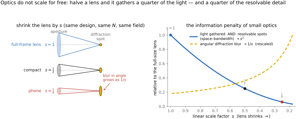
This explains the phone-camera limitation. A phone image looks worse than a full-frame image at low light not because its lens is badly designed (phone lenses are optical marvels, five to eight molded aspheres in a few millimeters) but because its aperture is small, and a small aperture is a small pipe for information. The engineering is excellent; the étendue is tiny. Much of computational photography on phones, including burst capture, multi-frame denoising, and learned upsampling, uses additional exposures and image priors to work within these limits. Bursts collect additional photons over time; learned detail can instead depend on a prior. Neither operation changes the single-exposure aperture or the diffraction limit.
22.6.1 Lohmann's scaling laws: why a good lens is heavy⧉
Lohmann's scaling analysis Lohmann 1989 separates geometric scaling from diffraction at a fixed wavelength. For a geometrically similar system, ray paths and transverse ray aberrations scale as $s$, while focal length and image size do too: geometric angular aberration is unchanged. Optical path-difference errors grow as $s$, so the same residual wavefront error occupies more wavelengths in an enlarged system. Meanwhile the diffraction spot at fixed f-number stays constant in physical size. This is why enlarging a design can expose aberrations that were hidden inside the diffraction spot at smaller scale.
| quantity, with fixed wavelength, f-number, and angular field | scale factor |
|---|---|
| focal length, pupil diameter, sensor width | $s$ |
| diffraction spot radius on the sensor | $1$ |
| angular diffraction blur | $1/s$ |
| diffraction-limited spatial cell count | $s^2$ |
| transverse geometric ray error and optical path-difference error | $s$ |
| volume and mass for similar shapes and materials | $s^3$ |
These exponents compare scaled copies, not all possible lens architectures. A redesigned prescription, a thin mirror, or a multiscale array need not obey the same mass-versus-aperture relation.
The practical tradeoff follows. Enlarging a well-corrected design raises its potential diffraction-limited detail count with area, but its glass volume rises faster, and its residual geometric blur can become large relative to diffraction. Shrinking it makes the geometric aberrations smaller in sensor units, yet diffraction does not shrink with them and the total collecting area falls. The miniature can be easier to correct optically while still carrying fewer resolvable spatial cells and fewer photons for a fixed output pixel count. Large cameras and telescopes therefore gain more than a longer barrel, but their designers must pay for correction, structure, and tolerances rather than simply scaling a finished prescription.
22.6.2 The gigapixel barrier for a single lens⧉
If you scale the system toward a very large image, the same laws create a different limit, this time from the cost side. Suppose you want a single monolithic lens that delivers a gigapixel: a billion resolved cells in one frame. The space–bandwidth product you need is enormous, so the aperture must be large (information is area), and the field of view must be wide. But a wide field at a large aperture is exactly the regime where aberrations are worst, and correcting them across the whole field demands more and more elements, each one larger, heavier, and more tightly toleranced than the last Cossairt, Miau & Nayar 2011. The volume grows as the cube of the size; the element count grows with the field; the cost and mass run away faster than the resolution you gain. There is a practical wall: beyond a certain space–bandwidth product, a single well-corrected lens becomes unbuildable. It is not impossible in principle, but it is impractical in glass, weight, and cost. A gigapixel image is not forbidden by physics, and there is no universal hard pixel-count boundary for monolithic optics. The difficulty is meeting a specified field, angular resolution, aperture, mass, and cost together.
This is the same trade-off that runs through the whole part (glass against computation, optics against architecture), but seen from the resolution axis rather than the quality axis. And the escape is the same in spirit: stop demanding that one lens do everything, and reorganize the system.
22.6.3 The escape: monocentric multiscale optics⧉
The way past the gigapixel wall is to split the problem. A large image needs a large aperture to collect the light, but it does not need a single large, perfectly-corrected lens to form the whole field at once. David Brady and colleagues built the alternative: a monocentric multiscale camera, in which one large shared objective does the light-gathering and a whole array of tiny micro-cameras does the correction and the sensing, each responsible for one small patch of the field Brady & Hagen 2009 Brady et al. 2012.
The shared objective is a monocentric ball: a sphere of glass (in practice a few concentric shells) whose every surface is centered on the same point. That symmetry is the trick. A monocentric lens has no preferred axis: every direction into it looks identical, so it forms a low-aberration image on a curved spherical surface, and it does so the same way for every field angle. It acts like a single large aperture with little field-dependent aberration to correct, but its image lands on a sphere, not a flat sensor, and it still carries the residual aberrations a single ball cannot fix. That is where the array comes in. Tiled across the curved focal surface sits a grid of small, cheap, identical micro-cameras, each a little relay lens plus its own small sensor. Each micro-camera re-images one small patch of the curved intermediate image onto its flat sensor and cleans up the residual aberration over its small field, and correcting a small field is easy and cheap, which is the whole reason small lenses can be excellent. The micro-cameras overlap slightly at their edges so their geometry and radiometry can be registered and blended. The shared objective reduces viewpoint differences relative to a widely spaced camera array, but does not eliminate the need to calibrate alignment, distortion, pupil geometry, or residual depth-dependent mismatch. Stitch the tiles and you have a gigapixel field assembled from dozens of small, individually sharp images: the resolution of a giant lens with the buildability of many tiny ones. These are Brady's AWARE cameras, demonstrations of gigapixel snapshot imaging Brady et al. 2012.
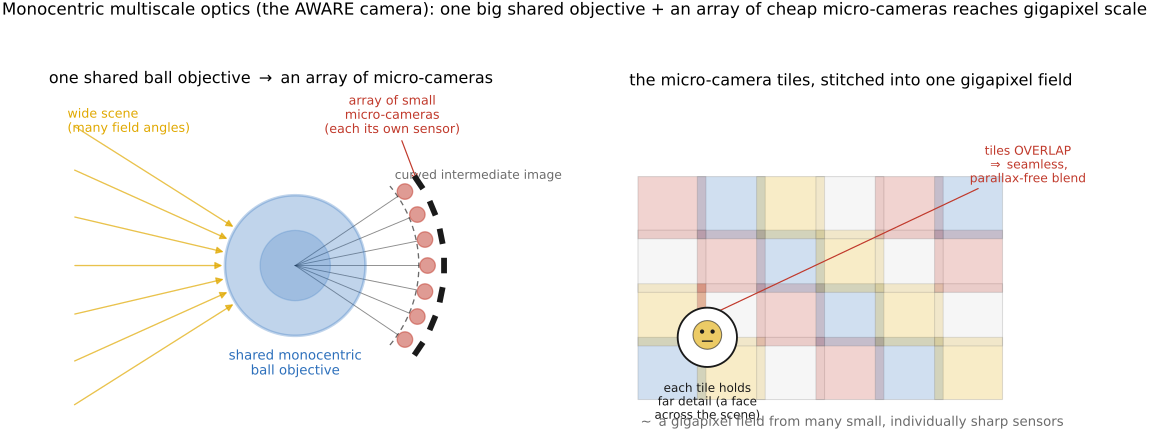
The architecture reduces the burden on a monolithic objective, while adding relay optics, sensors, alignment, electronics, and substantial computation and data handling. A gigapixel snapshot produces a very large data stream: dozens of sensors read out in parallel, their tiles geometrically aligned, color-matched, and blended across the overlaps into one seamless image, every frame. The architecture trades the impossible monolithic lens for a tractable optical system plus a serious stitching pipeline, which is exactly the optics-and-computation bargain the rest of this part keeps striking, here applied to the resolution wall instead of the aberration wall.
22.6.4 Capture everything, crop later: the spatial cousin of the light field⧉
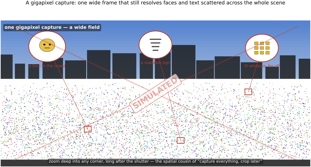
A gigapixel image gives you something closely related. The light field of the multi-aperture part lets you record the angular structure of light and then choose your viewpoint and your focus after the shutter: "capture everything, decide later" along the angular axis. A gigapixel field is the same bargain along the spatial axis: record the whole wide scene at fine resolution and choose your crop, framing, subject, and zoom after the fact. Both spend a sea of pixels to defer a decision from capture time to processing time; both run straight into the same data-rate wall, since a gigapixel per frame and a light field per frame are potentially large streams whose actual rates depend on spatial and angular samples, bit depth, and frame rate. They are cousins. The camera arrays of Part 31, Light fields and plenoptic cameras tile angle; the monocentric multiscale camera tiles space; and the deep reason either one needs an array at all is the scaling law of this chapter: a single small aperture cannot carry the information, so you build an architecture out of many.
Optical scaling changes diffraction, geometric aberrations, collecting area, and mass at different rates. The resulting compromises motivate architectures such as monocentric objectives with local relay cameras. Computation helps combine and interpret their measurements, while optical design still determines the available photons and spatial detail.