21.1 Inpainting, texture synthesis, and object removal⧉
Erase a person from a holiday snapshot and you are left with a person-shaped hole, a region of pixels you never photographed, surrounded by sand and sea you did. What should go in the hole? There is no measurement to consult; the camera recorded nothing there but the person who is now gone. And yet you have a strong sense of what should be there: more sand, more sea, the horizon line continuing unbroken from one side of the hole to the other. The visible sand, sea, and horizon constrain the answer; your prior, an internal model of beach photographs, explains how to continue them through the hole. Neither tells you whether an unseen shell or footprint lay behind the person.
This is the cleanest illustration in the whole book of the lesson that ran through super-resolution and deblurring: when the measurement genuinely gives you nothing, no amount of cleverness recovers it from the data, and a prior is what selects an answer. Super-resolution had to invent high frequencies the sensor folded away; inpainting has to invent whole regions. Here the problem is extreme: inside the hole there is zero data, so the fill depends on the prior conditioned on the visible context. It can be plausible without matching the hidden scene.
The chapter is one spectrum. At the weak end, a smoothness prior simply continues the surrounding color and edges inward: wonderful for a thin scratch, hopeless for a large hole. Stronger is a self-similarity prior that copies patches from elsewhere in the same image, which is what makes texture synthesis and object removal work. Stronger still is a database prior that pastes from other images entirely: a large photo database provides the prior. And at the strong end sits a learned generative prior that has compressed millions of images into weights and simply generates a completion. These families use progressively broader sources of information; we examine them in that order.
The prior is not optional, and filling a hole is the purest case. There is zero data inside the hole, so 100% of the answer comes from the prior. Smoothness, self-similarity, a photo database, a learned net: each is a different prior, and the result is exactly as good (and as truthful) as the prior is. The split that organized super-resolution survives intact: a prior is reconstruction-leaning where it copies genuine structure from somewhere real, and hallucination where it invents detail that was never anywhere. (Registered as L7.8; developed in Chapter 14.1, What can super-resolution actually do?; here taken to its extreme: no data, all prior.)
21.1.1 Inpainting as filling unmeasured pixels: the spectrum of priors⧉
State the problem plainly. We are given an image $I$ with a masked region $\Omega$ (the hole) marked by the user or by a defect detector, and we want a complete image in which $\Omega$ is plausible and seamless: the eye should not be able to find it. The defining feature is the one we keep returning to: there is no data in $\Omega$, so the fill is inferred from context under a prior, rather than read from a direct measurement. The only thing the algorithm has to work with is the known surround and whatever assumptions it makes about how the hole relates to it.
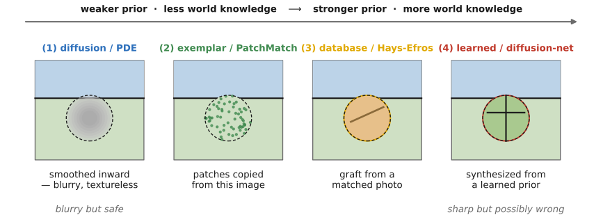
Read that way, the four families of methods are just four different answers to the question "what does the missing region look like?" (Figure 21.1.1):
- It looks like its immediate neighbors. Continue the surrounding color and edges smoothly into the hole. This is the smoothness / PDE prior, the weakest. It is superb for thin gaps, where the two sides are close and there is little to invent, but it blurs anything large, because pure smoothness has no notion of texture.
- It looks like some other part of this image. Images repeat themselves (grass is grass, brick is brick) so copy patches from elsewhere in the same image. This is the self-similarity / exemplar prior, the workhorse: texture synthesis, the clone and healing brushes, Criminisi object removal. It copies real structure (so it leans toward reconstruction) but only structure the image already contains.
- It looks like some other image. If this image does not contain the right content, perhaps another one does. Retrieve a matching scene from a vast database and graft a region in. This is the database prior (Hays & Efros), where the prior is, quite literally, the rest of the internet.
- It looks like a typical image. A network that has internalized the distribution $p(\text{image})$ can simply generate a completion that is plausible for images in general. This is the learned generative prior, the strongest and most flexible, and for exactly that reason the most prone to hallucinate.
Those four assumptions (looks like (a) its neighbors, (b) another part of this image, (c) another image, (d) a typical image) are the four families, with increasing flexibility rather than a formal ordering of statistical prior strength. The rest of the chapter walks the ladder. Treat it plainly: the algorithm is answering a question it has no data for, by assuming the hole resembles one of those four things.
21.1.2 PDE / diffusion-based inpainting⧉
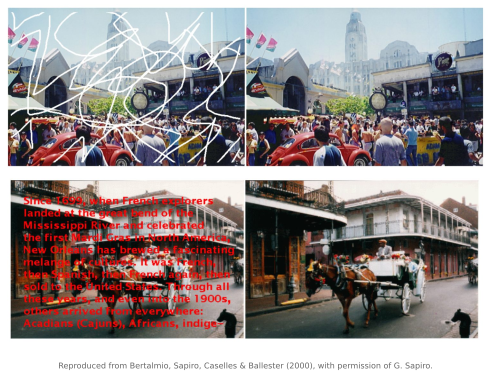
The weakest rung borrows its idea from the art world. A museum conservator repairing a cracked painting does not invent new subject matter inside the crack; she continues the lines that arrive at its edges, carrying a contour or a brushstroke smoothly across the gap so the eye glides over it. Bertalmío, Sapiro, Caselles and Ballester 2000, in the paper that named image inpainting, made exactly this into an algorithm.
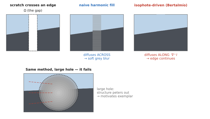
The naive version of "be smooth" is to solve Laplace's equation inside the hole, filling $\Omega$ with the harmonic function that interpolates its boundary values, the soap-film membrane we met in Chapter 10.8, Poisson image editing. That diffuses color inward, but it diffuses it in all directions equally, so an edge arriving at the boundary is smeared across into a soft blur rather than continued as an edge. The conservator's instinct is the opposite: diffuse along the contour, not across it.
Bertalmío's method encodes that instinct. The level-lines of an image (the curves of constant intensity, called isophotes) are perpendicular to the gradient $\nabla I$, so the direction along an isophote is $\nabla^\perp I$ (the gradient rotated by ninety degrees). The method propagates the image's smoothness (concretely, its Laplacian $\Delta I$, a local measure of intensity curvature) along those level-lines:
Read it back: push the smoothness information in the direction the level-lines run. An edge that meets the hole is an isophote; following it carries the edge straight across the gap instead of blurring it out. The original method alternates this transport with stabilizing diffusion. Run the coupled evolution and the hole fills with colors and contours that continue what surrounds it (Figure 21.1.2). Telea 2004 gave a different fast method built on fast marching and local intensity extrapolation, sweeping inward from the boundary in one pass instead of iterating a PDE to convergence, a related boundary-inward strategy, cheap enough for interactive scratch removal.
This works well for thin structures (scratches, scanner dust, text overlays, hairline cracks) where the two sides of the gap are close and there is genuinely little to invent: continuing the lines is almost as good as having measured them. But it has a hard ceiling. For a large hole there is nothing to propagate inward except flatness; the isophotes peter out long before they reach the center, and the fill goes blurry and textureless. Diffusion knows how to continue an edge but has no concept of texture: it cannot manufacture the grain of grass or the speckle of gravel, because those are not smooth at all. That failure is precisely the motivation for the next rung.
This rung is related to the gradient-domain / Poisson family, although its nonlinear transport equation is not a Poisson solve (cross-ref Chapter 10.8, Poisson image editing, 💡 L10.4): seamless cloning edits the gradient field where it has a source to copy from, and PDE inpainting edits it where there is no source at all: it manufactures the gradients to integrate from a smoothness assumption rather than copying them.
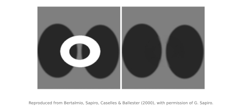
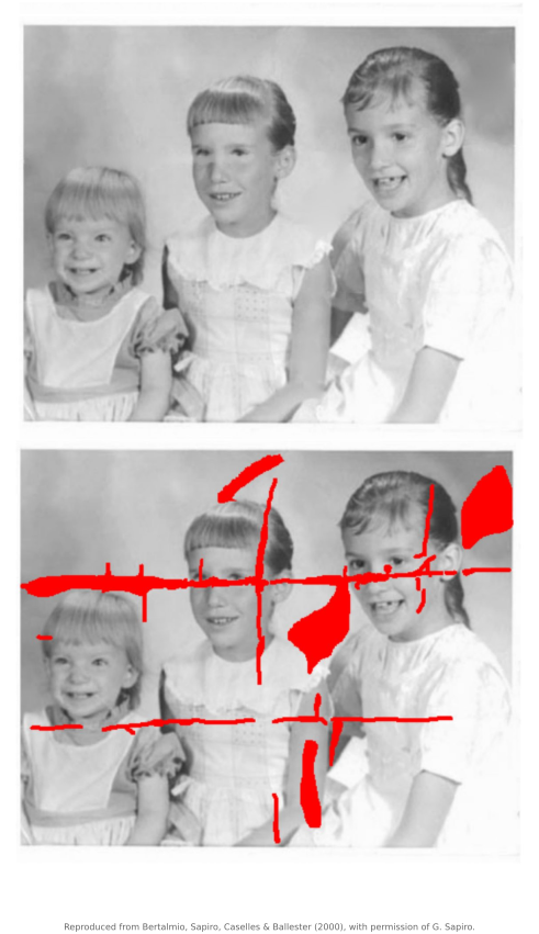
The original paper's own results make the same point on real and synthetic data.
21.1.3 Texture synthesis (Efros–Leung; Efros–Freeman quilting)⧉
The fix for a large hole in a textured region (grass, gravel, a knit sweater, foliage) is to stop trying to diffuse it and start trying to synthesize it. The useful observation is: texture is self-similar. A patch of lawn looks like every other patch of lawn; the missing piece is not smooth, but it is statistically a copy of what surrounds it. Use copied neighborhoods as an empirical model of the texture.
Non-parametric texture synthesis (Efros–Leung)⧉
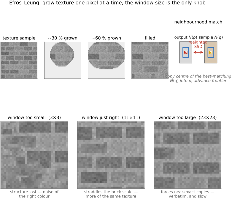
Efros and Leung's 1999 method Efros & Leung 1999 makes this idea literal: it synthesizes the texture one pixel at a time, and the sample image itself is the model: no parameters are fit at all. To fill the next unknown pixel $p$, take its already-known neighborhood $N(p)$ (the ring of pixels around $p$ that are already filled or were never missing) and search the source texture for windows that match it, scoring each candidate window $N(q)$ by a Gaussian-weighted sum of squared differences (SSD) over only the known part of $p$'s neighborhood. Pick a window that matches well, and copy its center pixel into $p$:
where $K_p$ contains the known offsets in the neighborhood, $w(u)$ is a Gaussian weight, $d_{\min}$ is the minimum candidate distance, and $\epsilon$ permits near-best matches. Thus the equation samples among matches just as the pseudocode does. Then $p$ is known, the frontier advances by one pixel, and you repeat:
while any pixel is unfilled:
    p ← unfilled pixel with the most known neighbours
    for each candidate window N(q) in the source:
        d[q] ← weighted mean squared difference over the known part of N(p)
    pick q at random among the windows with d[q] near the minimum
    Î(p) ← I(q)        # copy the matching window's centre pixel
In words: to decide what goes here, find the places in the image whose surroundings look most like this pixel's surroundings, and copy what they have in the middle. (Filling the most-surrounded pixel first keeps the synthesis frontier coherent; accepting a near-best match at random, rather than the single best, avoids verbatim repetition.) It is the Markov-random-field assumption made into an algorithm: a pixel's conditional distribution is modeled from its neighborhood, and the empirical distribution of "neighborhood → center" is the source image.
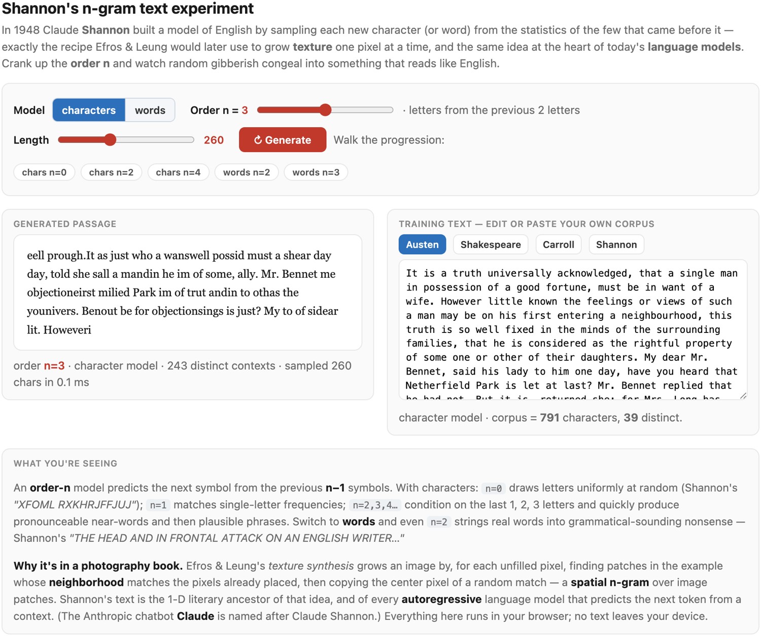
Efros and Leung's "copy a pixel by matching its surroundings" is, almost exactly, a fifty-year-old idea about text, and it traces to Claude Shannon, the engineer who founded information theory in 1948 (A Mathematical Theory of Communication), the paper that gave us the bit and the modern notion of information as something measurable. In that same work Shannon ran a now-famous toy experiment in generating English: build a table of which letter (or word) tends to follow the previous one, two, or three, then sample the next symbol conditioned on the last $n$, an $n$-gram model. With $n=0$ you get random letters; raise $n$ and the output slides from gibberish through pronounceable nonsense to almost-English ("THE HEAD AND IN FRONTAL ATTACK ON…"). The longer the context you condition on, the more structure appears, exactly Efros–Leung's window-size knob, one dimension over. The analogy is precise. Efros–Leung synthesizes a pixel by finding contexts in the source whose neighborhood matches the pixel's known surround and copying the center; Shannon synthesizes a letter by finding contexts whose preceding $n$ symbols match and sampling what comes next. Texture synthesis is Shannon's $n$-gram with the one-dimensional "previous $n$ letters" replaced by a two-dimensional spatial neighborhood: conditional sampling from the empirical distribution, in space instead of time. And the lineage runs straight on to the large language models of today, which generate text by sampling the next token conditioned on all the previous ones: the same conditional-sampling principle Shannon sketched, scaled up with a learned distribution in place of a lookup table. (Figure 21.1.6)
The main structural knob is the window size (Figure 21.1.7). Make it too small and the match sees only a few pixels, so it captures the texture's fine grain but loses any large-scale structure: bricks dissolve into a noisy mush of brick-colored speckle. Make it too large and the only windows that match are near-identical to the source, so the method copies the source verbatim, tiling it like wallpaper (and slowly, since each match is a full search). The window must straddle the texture's characteristic scale: large enough to see a whole brick, small enough not to lock onto one specific brick. That single trade-off (local randomness versus large-scale faithfulness) is the recurring theme of every patch method that follows.
The cost is speed: a full search over the source for every pixel is very slow, which is exactly the bottleneck Chapter 21.2, Patch match, later removes Barnes et al. 2009, and Wei & Levoy 2000 had already sped up by using fixed-shape neighborhoods amenable to tree search.
The paper's own figures show the mechanism and the knob on real textures.
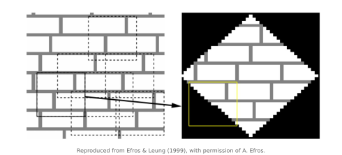
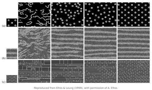
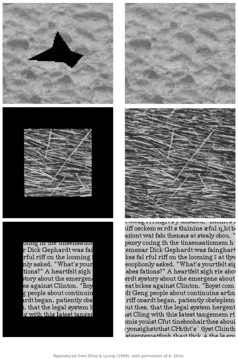
Image quilting (Efros–Freeman)⧉
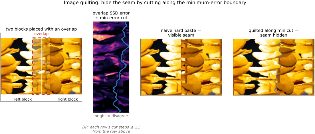
Synthesizing a single pixel per search is wasteful when whole patches of the source are reusable. Efros and Freeman's 2001 image quilting Efros & Freeman 2001 lays down overlapping blocks copied from the source, choosing each new block so that its overlap region matches what is already there. That alone would leave a visible seam wherever two blocks meet, so quilting adds a trick: in the overlap strip, it does not blend: it cuts along the minimum-error boundary, the path through the overlap where the two blocks disagree least, and takes one block on each side of the cut (Figure 21.1.11). Finding that least-disagreement path through a strip is a tiny dynamic program (a shortest path through a two-dimensional strip) and because the seam wanders through wherever the two patches happen to agree, it can become hard to see; a poor overlap match still leaves a visible seam.
Quilting is far faster than pixel-at-a-time synthesis (a whole block per search, not a pixel), and its min-error-seam idea is the direct ancestor of GraphCut textures (Kwatra et al. 2003 Kwatra et al. 2003), which generalize the one-dimensional cut to a full two-dimensional graph cut: place a patch and let min-cut/max-flow decide, per pixel, whether to keep the old texture or the new one, with the cut running along the seam of least visible disagreement.
That is not a coincidence; it is a big lesson. The patch-plus-min-error-seam view is discrete optimization on a graph, a match cost (how well a patch fits) plus a seam cost (how visible the boundary is), minimized by an off-the-shelf optimizer, with the energy doing all the design work.
The quilting seam is a graph cut; the energy is the design. Stitching two overlapping patches by choosing the minimum-error boundary through their overlap is exactly discrete optimization on a graph: a dynamic program in one dimension (quilting), a min-cut/max-flow in two (GraphCut textures, Kwatra et al. 2003). The optimizer is off-the-shelf; what you design is the energy: match cost (does this patch belong here?) plus seam cost (is the boundary visible?). The same machinery cuts panorama and photomontage seams and segments objects; texture synthesis is one more instance. (See L10.5, image edits as discrete optimization on a graph; first placed in Chapter 10.9, Seam optimization.)
Quilting places one block at a time. Texture optimization Kwatra, Essa, Bobick and Kwatra, 2005 instead improves every output patch at once: match each patch of the current output to its nearest exemplar patch, replace every pixel by the average of the matched patches that overlap it, and repeat, coarse to fine. The matching step is a nearest-neighbor field, which is why PatchMatch (Chapter 21.2, Patch match) made it fast. Adding a completeness term, so that every exemplar patch must also appear somewhere in the output, keeps the result from settling on the exemplar's plainest patches. The texture view of (Figure 21.2.8) runs this on an exemplar you drag over a photo.
A note on the road not taken: instead of copying patches, one can fit an explicit parametric model of the texture's statistics: Heeger & Bergen 1995 match the histograms of steerable-pyramid subband responses, and Portilla & Simoncelli 2000 match a larger set of correlations among those responses. Synthesize by coercing white noise to have the same subband statistics. These can struggle with some structured textures that patch copying preserves, but they are conceptually important: matching the statistics of multiscale filter responses is the direct ancestor of neural style's Gram-matrix idea (cross-ref Chapter 25.1, Style transfer, Chapter 6.6, Pyramids and wavelets).
21.1.4 Exemplar inpainting: clone, healing brush, and object removal (Criminisi)⧉
Texture synthesis fills a textured hole; exemplar inpainting turns the same patch-copying machinery on real photographs, where a hole sits among structured content (an edge, a horizon, a corner) that must continue across it. The lineage starts with two manual tools every retoucher knows.
The clone brush is the bare exemplar prior under hand control: pick a source region and paint its pixels into the hole. Pure copying betrays itself instantly: wherever the source and destination differ in lighting or color, a hard seam appears. The healing brush (Photoshop 7, 2002) fixes exactly that by transferring the source's texture and detail while re-matching the destination's color and illumination: its effect is related to transferring source gradients and adapting low frequencies to the surround, as in gradient-domain / Poisson editing (cross-ref Chapter 10.8, Poisson image editing, 💡 L10.4). The relationship is the one we already drew: Pérez, Gangnet & Blake's gradient-domain cloning Pérez et al. 2003 was inspired by the healing brush and gave it its clean formulation (Georgiev 2005 later recast it as a covariant-derivative correction).
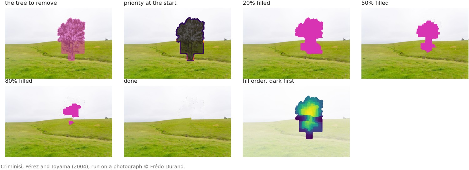
Criminisi, Pérez and Toyama 2004 automated the clone brush into full object removal. The texture-synthesis idea (copy the best-matching patch) is sound, but applied in a careless order it fails on the very thing that matters in photographs: linear structure. If you fill flat regions before edges, a wall's edge or a horizon line arrives at the hole from two sides and the two extensions do not meet; the structure breaks. Criminisi's contribution is a fill order that processes the hole's boundary in a deliberate sequence, by assigning each boundary patch a priority
the product of a confidence term $C(p)$ (how much of this patch's neighborhood is already reliably known, so we fill the most-surrounded regions first) and a data term $D(p)$, how strongly an image structure (an isophote, an edge) runs into the hole at $p$. The data term does the work: it pushes patches where a strong edge meets the boundary to the front of the queue, so linear structures are continued across the hole before the flat regions on either side are filled in (Figure 21.1.13). The effect is that a removed person's hole is closed by sand and sea that meet correctly at the horizon, not by two mismatched halves.
The limits are the limits of self-similarity itself: the search is slow and confined to this image's content. PatchMatch (Chapter 21.2, Patch match) removes the slowness, making the search interactive; a database (Hays & Efros) or a learned net removes the "only this image" ceiling.
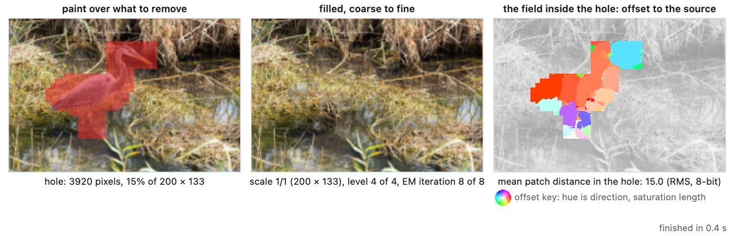
Criminisi's method fills the hole once, patch by patch, and a patch placed early is never revisited. The completion used with PatchMatch instead treats the whole hole as the unknown of one optimization and refines all of it at every iteration, from a coarse level of an image pyramid to the finest. The hole-filling view of the same figure paints the hole and shows the fill at every level.
21.1.5 Data-driven scene completion (Hays & Efros)⧉
Every method so far is trapped inside one image: if this photo does not contain the right grass, sky, or building façade, self-similarity has nothing to copy. Hays and Efros 2007 turned the simple idea of using another image into a system. To fill a hole, they retrieve, from millions of photographs, scenes whose surround matches the area around the hole, then take a good match, align it, cut a region out along a graph-cut seam, and Poisson-blend it into place. The completion is borrowed wholesale from a photo that was never of this scene at all.
The prior is a large image database. With a large enough database, some photograph already contains a plausible thing to put in the hole (a stretch of sky with the right clouds, a building wall of the right kind) so you retrieve the answer instead of modeling it. This is the non-parametric, copy-from-an-example prior taken to web scale: the exemplar is no longer a patch of this image but a region of some image.
The cost is steep: the grafted region is from a semantically different scene. The result is coherent and photoreal, but it is not this scene's truth: the clouds are real clouds, just not the clouds that were there. It is a clear demonstration of L7.8's "plausible ≠ measured." And it needs a genuinely huge database plus reliable scene matching to find a graft that fits.
Scene completion is also the conceptual hinge to deep learning. Both database retrieval and learned generation draw on collections of images. A generative network learns a distribution from its training data and can synthesize a completion without retrieving a particular stored photograph. Its generalization and failure modes therefore differ from nearest-neighbor retrieval, even when the two use similar training collections.
Scene corpus, the standard inpainting / scene-parsing set. <http://places2.csail.mit.edu>. See the Chapter 45.16, Datasets appendix.
21.1.6 Deep inpainting (context encoders → partial/gated conv → diffusion)⧉
The strong end of the ladder replaces the hand-built prior with a learned one (💡 L7.6, Chapter 7.3, Deep learning): a network trained to regenerate masked regions, having seen enough images to know what plausibly belongs in a hole.
Context encoders Pathak et al. 2016 were an influential early convolutional neural network (CNN) inpainting method, an encoder–decoder trained with a reconstruction loss plus an adversarial loss (a generative adversarial network (GAN) discriminator pressuring the fill to look real). They captured semantics that no copy-based method could (completing a face with a plausible eye, not a patch of skin) but early versions were blurry, because a reconstruction loss averages over the many plausible completions.
Partial and gated convolutions Liu et al. 2018; @yu-etal-2019|Yu et al. 2019 fixed a quiet but crippling nuisance: a vanilla convolution applied near a hole mixes the hole's garbage masked pixels into its output, poisoning everything downstream. Partial convolution renormalizes each output by the fraction of valid (known) pixels in its receptive field and shrinks the hole layer by layer; gated convolution goes further and learns a soft per-pixel mask gate. The result is that it handles free-form holes of any shape: the practical "select this object and remove it" workhorse behind modern editing tools.
A second fix targets the size of the hole. A network with a small receptive field cannot relate structures on opposite sides of a large mask. LaMa (Suvorov et al. 2022) uses fast Fourier convolutions to make global context available early, along with a loss with a large receptive field and large training masks. Its spectral branch is not merely an ordinary local convolution computed by FFT: it processes Fourier features and maps them back into spatial features. This helps with periodic structures and large masks, but does not guarantee a correct completion at arbitrary size. One-tap object-removal products use learned inpainting, sometimes with generative components, but their public interfaces do not establish that they use LaMa or any particular research architecture. Google's phone tools show the progression from the user's side: Magic Eraser (2021) removes a selected distraction and fills the hole with a plausible continuation of the background, while Magic Editor (2023) uses a generative model to fill larger regions and can also move or resize the subject, which requires synthesizing what was behind it. The common task is to detect or select an object, mask it, and synthesize a compatible replacement.
Diffusion inpainting Lugmayr et al. 2022, RePaint is the strongest prior and closes the loop back to Chapter 7.5, Image priors. Treat the hole as a measurement constraint (the known pixels are the measurement, the masked pixels are unknown) and run a pretrained diffusion model's denoising loop, but at every step pin the known region to the real pixels (renoised to that step's noise level) while letting the network fill the rest:
Here $M=1$ on known pixels, $q$ is forward noising to the indicated time, and $p_\theta$ is the learned reverse transition. RePaint also uses a resampling schedule with forward jumps and repeated reverse steps to improve agreement across the mask boundary.
This shares the separation of data constraints and learned image structure used in plug-and-play methods, but is not identical to RED optimization or a guarantee of exact posterior sampling (💡 L7.7) with the forward operator set to "keep the known pixels": the data-fit step re-injects the measurement, the denoise step imposes the prior, and the loop alternates, the same recipe as super-resolution and deblurring, with masking as the measurement. The architectures themselves live in Chapter 7.3, Deep learning / Chapter 7.4, Generative AI and diffusion; here they are simply the strong-prior end of the spectrum.
The caveat is strongest here, because this is where it bites: the learned prior is the most flexible and the most prone to hallucinate. It will confidently invent a face, a license plate, a sign's text that were never measured and may be wrong. An inpainted region is not evidence, a forensic and ethical line this part has drawn since super-resolution L7.8.
21.1.7 Highlight / specular recovery⧉
A last, less obvious instance closes the chapter, because it is inpainting in disguise. A blown highlight (a glaring specular spot on metal, a sky clipped to pure white, a sunlit window) is a region where the sensor saturated: one or more channels reached their ceiling, so the value above that threshold was not recorded. Saturation still supplies a lower-bound constraint, so a clipped region is not quite an unconstrained hole, and highlight recovery is inpainting it: filling the saturated pixels with a plausible surface color using the surroundings and whatever was not clipped as the prior (Figure 21.1.14).
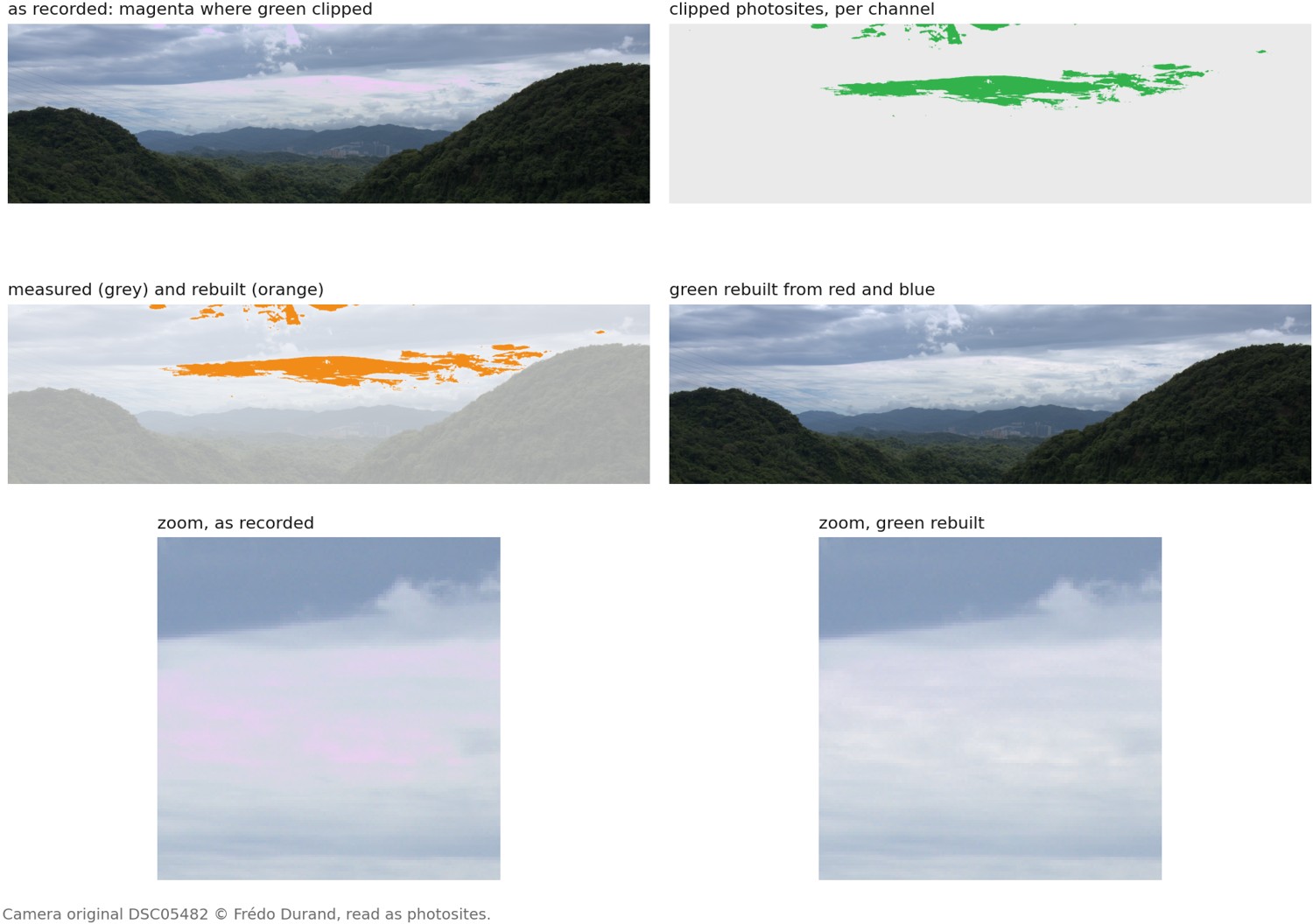
There are two complementary angles. The first is specular–diffuse separation: a highlight is the specular reflection added on top of the underlying diffuse surface, so recovering the diffuse layer beneath it is the goal (cross-ref the illumination-in-a-single-image material). The second, and more directly inpainting-flavored, is per-channel clipping recovery: highlights rarely clip all three color channels at once, so when only the red channel has saturated, the unclipped green and blue still carry two channel measurements and local structure, but do not determine the missing red or full hue, and the missing red can be extrapolated from them and from the surround, a more constrained but still ambiguous inpainting whose prior is "the channels move together."
It lives here for the same L7.8 reason as everything else: recover what the measurement destroyed, destroyed by clipping rather than by masking, but unmeasured all the same. And it has a grounded, non-inpainting cousin: rather than guess the highlight, capture it with a shorter exposure and merge, the high-dynamic-range (HDR) move of trading a guess for a measurement (forward-ref Multiple exposure imaging). Inpainting the clip is what you do when you only have the one frame.
21.1.8 Epitomes: a compact patch model⧉
The exemplar methods above treat the image itself as the dictionary of patches to copy from. Epitomes (Jojic, Frey & Kannan 2003) instead learn a miniature (an "epitome" a fraction of the image's size) fit so that every patch of the original has a close match somewhere inside it. It is a generative patch model: the full image is explained as a quilt of overlapping epitome patches, and the usual tasks fall out of "find each patch's place in the epitome and read back a clean (or completed) version": denoising, inpainting, super-resolution, texture transfer. It is the same patch-nearest-neighbor idea that drives texture synthesis and Chapter 21.2, Patch match, but with a learned, compact dictionary in place of the raw image, and so the pre-deep cousin of today's learned patch and latent priors (L7.6 / L7.7), a bridge from exemplar copying to the modern generative models of Chapter 7.4, Generative AI and diffusion.
The Remove tool of Chapter 8.13, A raw developer in the browser is this chapter's machinery at interactive size: click a blemish, and source selection plus a feathered fill do what the pseudocode here says.
Recap: big lessons of this chapter
The prior is not optional, and filling a hole is the purest case. There is zero data inside the hole, so 100% of the answer comes from the prior. Smoothness, self-similarity, a photo database, a learned net: each is a different prior, and the result is exactly as good (and as truthful) as the prior is. The split that organized super-resolution survives intact: a prior is reconstruction-leaning where it copies genuine structure from somewhere real, and hallucination where it invents detail that was never anywhere. (Registered as L7.8; developed in Chapter 14.1, What can super-resolution actually do?; here taken to its extreme: no data, all prior.)
The quilting seam is a graph cut; the energy is the design. Stitching two overlapping patches by choosing the minimum-error boundary through their overlap is exactly discrete optimization on a graph: a dynamic program in one dimension (quilting), a min-cut/max-flow in two (GraphCut textures, Kwatra et al. 2003). The optimizer is off-the-shelf; what you design is the energy: match cost (does this patch belong here?) plus seam cost (is the boundary visible?). The same machinery cuts panorama and photomontage seams and segments objects; texture synthesis is one more instance. (See L10.5, image edits as discrete optimization on a graph; first placed in Chapter 10.9, Seam optimization.)