20.4 Bells and whistles⧉
A long panorama exposes errors that a two-image stitch can hide: accumulated alignment drift, lens distortion, inconsistent brightness and moving content. Use overlap constraints across the image set, then choose a projection and source masks appropriate to the scene.
Keeping the source frames lets the final projection, crop and moving-object selection remain editable (L13.1).
The shift from a chain of pairwise estimates to a solve over the overlap graph is useful beyond panoramas. Structure-from-motion and simultaneous localization and mapping also use repeated observations to constrain a camera trajectory globally. A loop supplies information that a purely forward chain cannot use: the view at the end must agree with a view seen earlier.
20.4.1 Other projections⧉
A panorama can span far more of the world than a single flat image plane can hold, which forces a question the two-image demo never had to ask: onto what surface do you unroll the mosaic? The frames have already been registered to one another by the homographies; choosing a projection is a separate, later step, a re-parameterization of the output canvas, independent of the alignment. But it is not a cosmetic choice. The surface you pick decides what looks natural and what distorts, and there is a hard geometric tradeoff that no cleverness escapes.
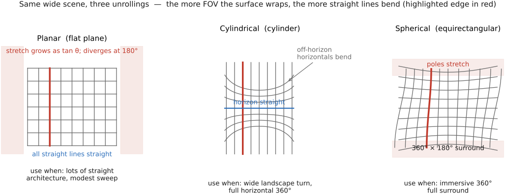
Planar, or rectilinear, projection keeps scene lines straight under the central-camera model. It can approach but not reach a 180-degree field of view in a finite image; stretching becomes severe well before that. A 120-degree limit is a practical preference, not a mathematical cutoff.
Cylindrical projection can cover a full horizontal turn. With a level vertical axis, vertical scene lines and the horizon remain straight, while many other lines curve. Output scale is a rendering choice; calibrated intrinsics are needed to convert source pixels into rays.
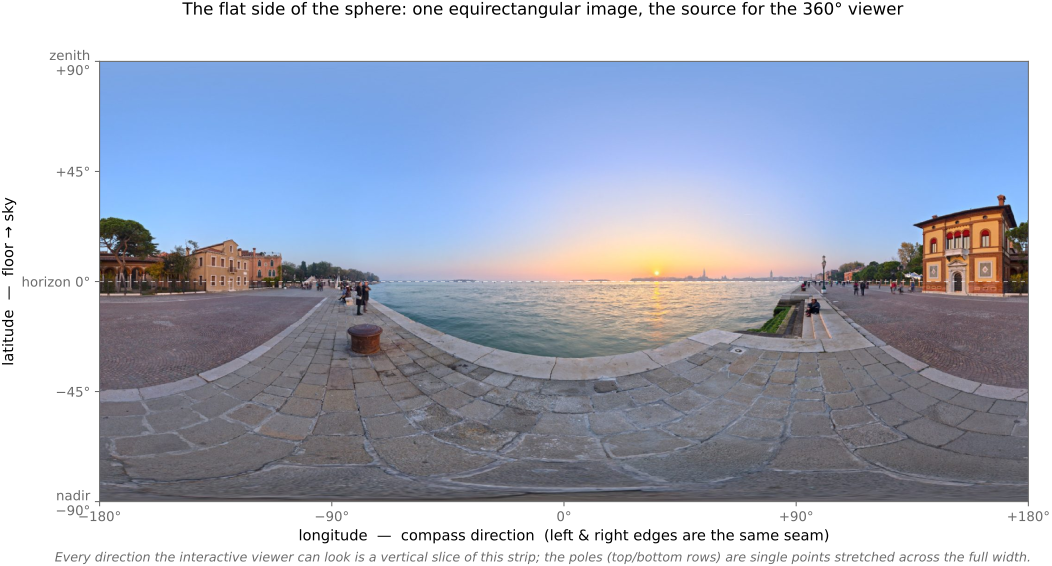
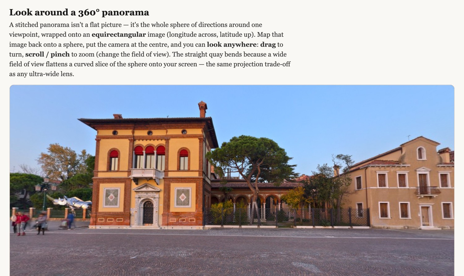
An equirectangular image stores longitude and latitude on a rectangular grid, commonly covering 360 by 180 degrees in a 2:1 image. It is one representation of spherical directions; cube maps are another. The poles have singular coordinates and increasing area distortion. An interactive viewer resamples these directions into a perspective viewport, where correctly reconstructed straight scene lines remain straight.
For a camera ray $d=(d_x,d_y,d_z)$ with vertical axis $y$, define
Equirectangular coordinates are proportional to $(\theta,\phi)$, while cylindrical coordinates are proportional to $(\theta,d_y/\sqrt{d_x^2+d_z^2})$. Choose pixel scale, origin and vertical sign explicitly. Both need longitude wrapping; cylindrical projection is undefined at the vertical poles.
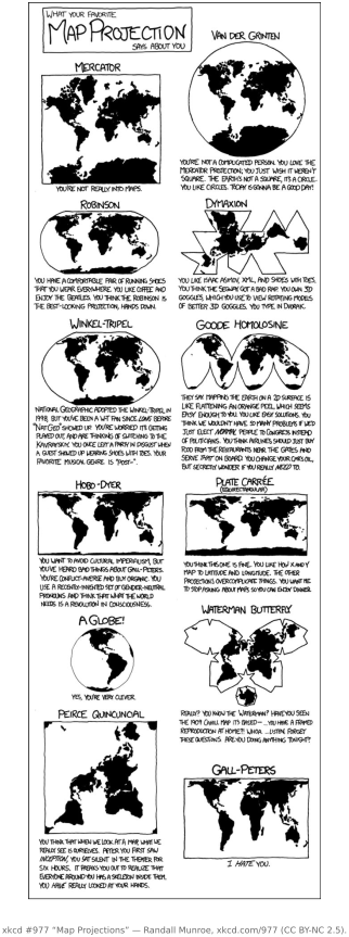
The pattern across the three is one tradeoff stated plainly, and it is unavoidable: you cannot simultaneously cover a very wide field of view and keep all straight lines straight on a flat output. This is the cartographer's dilemma: you cannot flatten a sphere onto a plane without distortion, which is why every world map lies about something (areas, angles, or distances). Planar buys straight lines at the cost of field of view; cylindrical and spherical buy field of view at the cost of bent lines. So pick by content: lots of straight architecture and a modest sweep favor planar; a wide landscape turn favors cylindrical; an immersive 360° surround demands spherical (Figure 20.4.2). Cartographers face the very same menu of compromises (Figure 20.4.1).
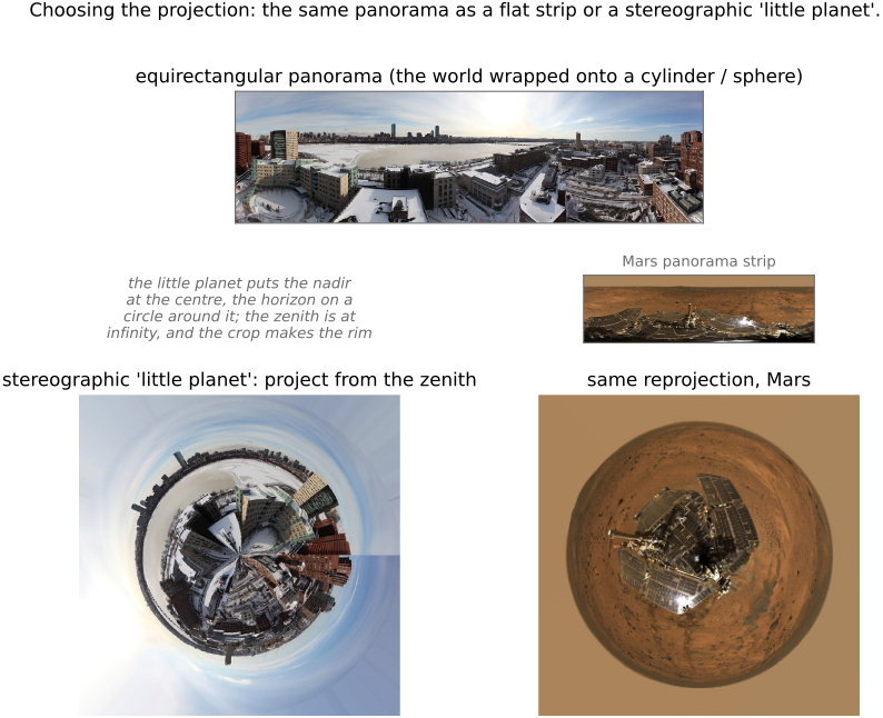
Because the projection is just a re-parameterization of the output canvas, nothing stops you from choosing a deliberately creative one. The stereographic "little planet" projects a full $360°$ panorama from the zenith down onto a plane, wrapping the horizon into a circle and curling the ground into a tiny world seen from above: the same registered mosaic, unrolled for effect rather than fidelity. It is the playful end of the same freedom bundle adjustment and blending exist to protect.
An equirectangular map and a perspective viewer represent the same directions differently. The horizontal coordinate wraps in longitude; the poles collapse many coordinates onto one direction. A perspective viewport samples a curved footprint in that map, not a rectangular vertical slice. Street-level map imagery is the familiar case. A vehicle-mounted rig records a full sphere of directions at each stop, the panorama is stored in a spherical format, and the browser shows a perspective window into it that follows the viewer's drag. Moving to the next stop loads the next panorama rather than moving within one; the change of viewpoint between stops is parallax, which a single panorama cannot represent.
20.4.2 Bundle adjustment⧉
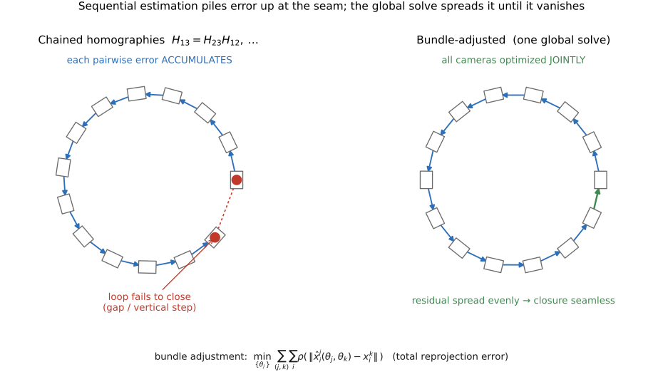
The naive pipeline builds a multi-image panorama the obvious way: it estimates each homography between adjacent frames and composes them to relate distant frames: $H_{13} = H_{23} H_{12}$, and so on around the sequence. Each pairwise homography carries a small estimation error, and composing a chain of them accumulates those errors. The symptom is unmistakable on a closed loop: shoot a full 360° panorama and, by the time the chain comes back around to where it started, the two ends do not meet, and there is a visible gap or vertical step at the closure (Figure 20.4.6). Sequential estimation lets error pile up and dumps the whole accumulated discrepancy at the seam.
Joint camera optimization uses all verified overlap constraints rather than committing permanently to pairwise estimates (Brown & Lowe 2007; Triggs et al. 2000). It distributes residuals according to geometry, confidence and loss, not necessarily evenly. Inconsistent data or an incorrect motion model can still leave a visible closure error.
Let $R_j$ map camera-$j$ rays to a common world frame. Predict a match from image $j$ in image $k$ by $\hat x_{ik}=\pi(K_kR_k^{\mathsf T}R_jK_j^{-1}\tilde x_{ij})$, including distortion in the projection functions when modeled. Fit the observed two-dimensional positions $x_{ik}$:
The solve minimizes match residuals over the connected overlap graph. Fix one camera orientation to remove the global-rotation gauge; constrain calibration parameters that the data cannot determine reliably. Initialize from validated pairwise estimates and use nonlinear least squares with a declared outlier-resistant loss. A global formulation is not a global-optimum guarantee.
Geometric reprojection residuals do not constrain exposure gains. Photometric consistency needs a separate term using valid, corresponding image intensities. Geometry and photometry can be solved jointly or in alternating stages; both designs can work.
The first is gain (exposure) compensation. Frames shot around a panorama rarely share an exposure exactly (auto-exposure drifts, the sun moves behind a cloud), so the overlaps disagree in brightness. Assign each image a per-image gain $g_j$ (and optionally a per-channel white balance) and choose the gains so that overlapping pixels agree photometrically:
The first term pulls the overlapping brightnesses into agreement; the regularizer $\lambda \sum_j (g_j-1)^2$ keeps every gain near 1 so the whole panorama does not drift uniformly dark or bright (the trivial all-zero solution that the first term alone would happily accept). Solving this before the seam blend removes most of the exposure mismatch up front, which is exactly what makes the blending of the previous chapter easy, because a blender hides a small residual mismatch far more gracefully than a large one.
The second is vignetting, the radial brightness falloff that darkens a lens's corners relative to its center. A per-lens falloff model is estimated jointly so that the same scene point matches in brightness whether it happens to land at the center of one frame or the corner of the next. And one can fold in radial distortion as well: the barrel or pincushion warp that bends straight lines near the frame edge, modeled as
with the distortion coefficients $\kappa$ added to the per-camera parameters $\theta_j$ so that straight scene lines align across frames rather than fighting the homography at the seams. (The distortion model itself is developed in Chapter 22.2, Aberrations correction; here it is simply another set of unknowns in the global fit.)
Check geometric residuals and photometric residuals separately. Fixing gauges, rejecting invalid overlaps and calibrating lens behavior matter more than whether the implementation is described as one solve or several.
20.4.3 Movement and parallax handling⧉
The previous two sections repaired the geometry and photometry of the panorama while still assuming two things the world routinely violates: that the scene is static, and that the camera only rotated. This section is what happens when each of those assumptions breaks. The first failure, something moved between frames, is fixed by a tool you already have. The second, the camera translated, is a genuine limit of the homography model, and worth understanding precisely so you know when to stop fighting it.
Deghosting: one source per moving region⧉
After background alignment, moving subjects can remain displaced. Local correspondence can align some of them, but occlusions and differing exposure blur leave unsupported regions. Source selection is another option; it needs a policy for which moment to show.
Large overlap differences flag inconsistency, which can come from motion, parallax or photometric error. Use those diagnostics and, where needed, object masks or user constraints to prefer a coherent source for each subject.
Source selection is the seam-optimization problem of Chapter 10.9, Seam optimization with one extra consideration in the cost. Recall the seam energy from Chapter 20.3, Blending, $E = \sum_p D_p + \sum_{pq} V_{pq}$: a per-pixel data cost $D_p$ for the frame each output pixel is drawn from, plus a smoothness cost $V_{pq}$ for switching frames between neighbors. Deciding which frame supplies each moving region is exactly such a per-pixel labeling. Make the smoothness cost high where the aligned frames disagree, so that cutting through a moving blob is expensive and cutting around it is cheap, and a graph-cut optimizer (Boykov, Veksler and Zabih, 2001) routes the seam around the object, then the pyramid or Poisson machinery of Chapter 6.6, Pyramids and wavelets and Chapter 10.8, Poisson image editing blends along it (Figure 20.4.8). Deghosting is the blending chapter's seam energy with motion disagreement folded into the cut cost: the energy is the design.
A seam energy can discourage cuts through a moving region, but ordinary local costs do not guarantee a whole object receives one label. Enforce that requirement explicitly when it matters. Removing all copies of a passerby also requires background observations to fill the uncovered area.
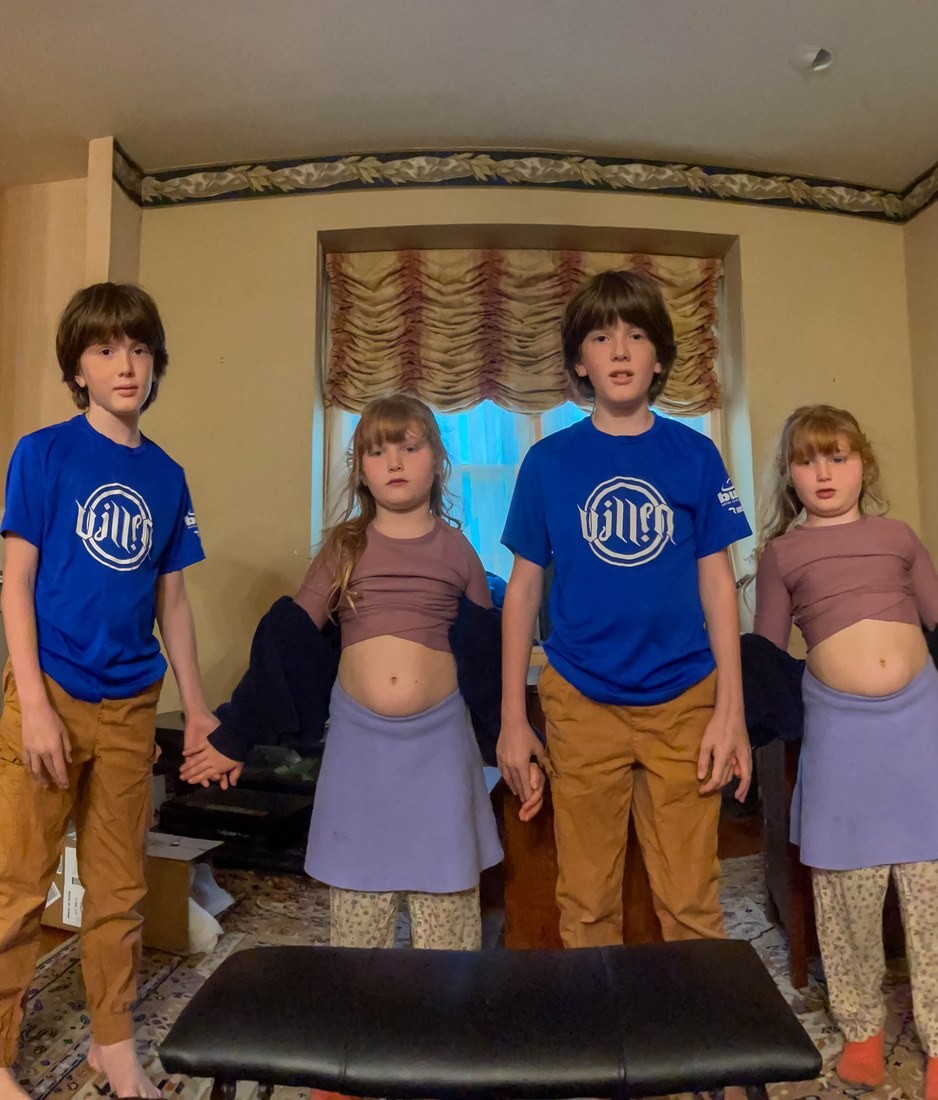
The multiplicity case is also the easiest to cause on purpose (Figure 20.4.7). A phone's sweep panorama builds the image from a continuous series of slices as you pan; if a subject runs behind the camera and back into a not-yet-captured part of the sweep, they are photographed more than once, landing in the panorama several times over. Two children who keep darting to the far end of the pan become four, or six: the static-scene assumption broken deliberately instead of repaired.
Parallax: when translation breaks the homography⧉
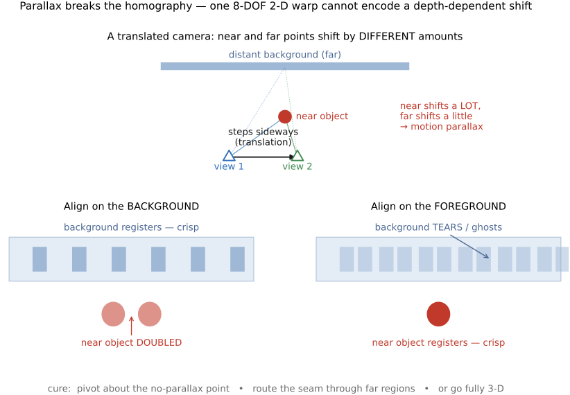
The deeper limit is geometric, and it is not a bug to be tuned away. Recall from Chapter 20.1, Manual panorama stitching from multiple views why a homography can align two frames in the first place: it is exact under a central-camera model for pure rotation about the projection center or points on a plane; a very distant scene can make translation effects negligible. Under pure rotation every scene point, near or far, moves between the two views by the same projective map, which is what let a single $3 \times 3$ homography $H \simeq K R K^{-1}$ stand in for the whole scene, with no dependence on depth.
The moment the camera translates (the photographer takes a step sideways), that guarantee collapses. Now near and far objects shift by different amounts: this is motion parallax, the everyday effect by which nearby fence posts streak past a train window while distant mountains barely move. And no single homography can align both: line up the background and the foreground doubles; line up the foreground and the background tears (Figure 20.4.9).
Translation makes correspondence depend on scene depth, so one projective transform generally cannot describe the whole overlap. A local displacement field can encode that variation where correspondence exists; a single global homography cannot.
Because the limit is structural, the practical escapes either avoid the translation or stop using a homography:
- Rotate about the no-parallax point. If the camera pivots about its entrance pupil viewpoint translation is reduced under a central-camera approximation and the homography is once again valid. This is precisely why tripod panoramas use a nodal slide to position the lens's pupil over the axis of rotation.
- Accept it locally. Route the seam through low-parallax regions (distant sky, uniform wall) using the graph cut once more, and blend, so that the unavoidable mismatch is hidden where the scene is far away or featureless enough that no one notices.
- Go 3-D. When translation is essential to the shot, abandon the single-homography model and estimate scene depth with genuine multi-view geometry (Hartley and Zisserman). This is the hand-off to structure-from-motion and to Matching pixels across space and time, where a per-pixel, depth-aware warp replaces the one global map.
A handheld sweep may include viewpoint translation and rolling-shutter motion. Their magnitude depends on capture, and narrow strips can conceal some mismatches without making the underlying central-camera assumptions exact.
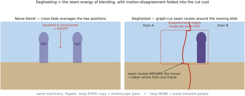
Source selection makes several different composites possible. In an overlap containing a walking person, assigning the whole person to one frame can avoid a translucent double exposure. Choosing separate complete appearances can intentionally make a sequence-of-motion composite. Removing the person altogether requires some source to show the background behind each removed region. A seam cost can favor cuts around the person, but if keeping an object whole is a requirement, that requirement must be encoded rather than assumed to follow from local smoothness. Blend after selecting content; blending alone cannot decide which event the panorama should depict.