20.3 Blending⧉
Two registered views can still disagree in exposure, color or vignetting. Residual parallax and moving subjects may also remain. Inspect geometry before blending: a smooth transition can conceal a brightness step, but it cannot make two displaced copies of an object coincide.
Choose source regions and transition widths according to the remaining mismatch. Feathering, multiscale blending and gradient-domain reconstruction offer different controls; they are not an ordering from universally inferior to superior methods.
A source change can introduce an edge that was absent from the scene. Blending reduces that discontinuity or moves the transition to a less conspicuous location. Smooth brightness and color errors can remain visible, so inspect the whole image as well as the seam.
Keep the original frames and editable source masks so the final choice of content and blend can be revised (L13.1).
20.3.1 Why a hard seam is visible: the photometric mismatch⧉
Registration provides a common coordinate system, but residual geometry can remain. Photometric differences include:
- Exposure / auto-exposure drift. The camera re-meters between shots (or you nudged the shutter or ISO), so the same wall is brighter in one frame than the next.
- White-balance drift. Auto white balance shifts per frame, leaving a color cast that differs across the seam.
- Vignetting. Lens shading often darkens the corners, so the same scene point is darker when it lands near a frame edge than when it lands at the center, which can produce disagreeing brightness ramps across the overlap.
A hard source switch can turn a brightness mismatch into a visible step. A broad transition may be less conspicuous, but it can still appear as shading or a color band. Correct systematic exposure and lens falloff before asking the blend to hide them.
Use common linear-light values for a radiometric weighted average. The overlapping images are alternative measurements, not independent light sources being added. Appearance-oriented gradient or pyramid operations can use another declared domain, but their result then follows that rendering objective rather than a radiance average.
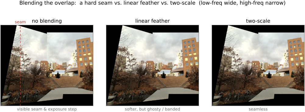
A hard source cut is a useful baseline and can work well where images agree. Blending is needed when the chosen boundary leaves a visible mismatch.
20.3.2 Feathering / alpha blending, and why it ghosts⧉
The first real idea, smooth blending, is to make each output pixel a weighted average of the sources, with each source's weight falling off toward its own frame boundary:
A source counts fully in its interior and fades to zero at its edge, so the transition is gradual and the seam softens into a cross-fade rather than a step.
A source-space ramp is inexpensive and can be warped with the image, although it is not the exact distance to the warped boundary. Multiply weights by valid coverage, accumulate weighted color and total weight, and normalize only where that total is positive. Keep uncovered output transparent or explicitly invalid. When filtering near source borders, carry associated color and coverage together to avoid blending invalid black into the image.
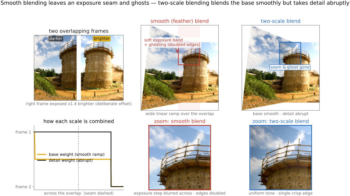
Feathering averages residual misalignment as well as noise. A wider transition can spread doubled edges over a larger area. Narrowing it reduces mixed content but may expose a brightness step or cut through an object.
The diagnosis is what motivates everything that follows. Feathering uses one transition width for all frequencies. But the right width is frequency-dependent: the low frequencies, such as the exposure and vignetting ramp we actually want to merge, need a wide, smooth blend; the high frequencies, the sharp detail we want crisp and un-ghosted, need a narrow, almost-abrupt transition. One width cannot serve both. That single realization is the entire rest of the ladder.
For three overlapping frames, keep one weighted-color accumulator and one weight accumulator. For each valid warped sample, add its color times its weight to the first and its weight to the second. Divide only after all frames have contributed. A location covered by three equally weighted samples then averages three samples, rather than averaging the third sample with an already averaged pair and giving it twice their individual influence.
A weight ramp can be constructed in each source rectangle and warped with the image. It provides a convenient fade toward the source borders, although after a projective warp it is not generally the Euclidean distance to the boundary in output pixels. Carry a separate validity mask so samples outside the captured image do not darken the accumulator.
20.3.3 Two-scale blending: the simple split (the pset method)⧉
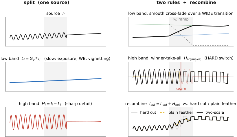
A useful teaching approximation splits each image into two bands and blends them differently. It illustrates multiscale blending without requiring a full pyramid.
- The low band $L_i = G_\sigma * I_i$ (a Gaussian blur) carries exposure, white balance, and vignetting, the slow stuff we want to merge smoothly. Smooth-blend it with the feathering weights above. A wide transition spreads the low-frequency mismatch gradually, although a visible brightness band can remain.
- The high band $H_i = I_i - L_i$ (the residual detail) carries the sharp edges and texture. Here a smooth average is exactly what causes ghosting, so we do the opposite, winner-take-all: at each pixel keep the high-frequency detail from the single source with the highest weight,
Selecting one high-band value avoids averaging two values at that pixel. It does not guarantee a single intact object: the selected source can change across the object, and its low-frequency contribution can still be mixed.
Recombine by addition, $I_{\text{out}}=L_{\text{out}}+H_{\text{out}}$. This can reduce feathering blur, but inspect seams where the selected high-band source changes and low-frequency ghosts around moving objects.
This two-band teaching method is related to pyramid blending, but winner-take-all detail is not identical to a conventional two-level Gaussian-mask blend. More bands allow additional transition scales; they do not repair incorrect registration.
20.3.4 Multiband / Laplacian-pyramid blending: a transition per band⧉
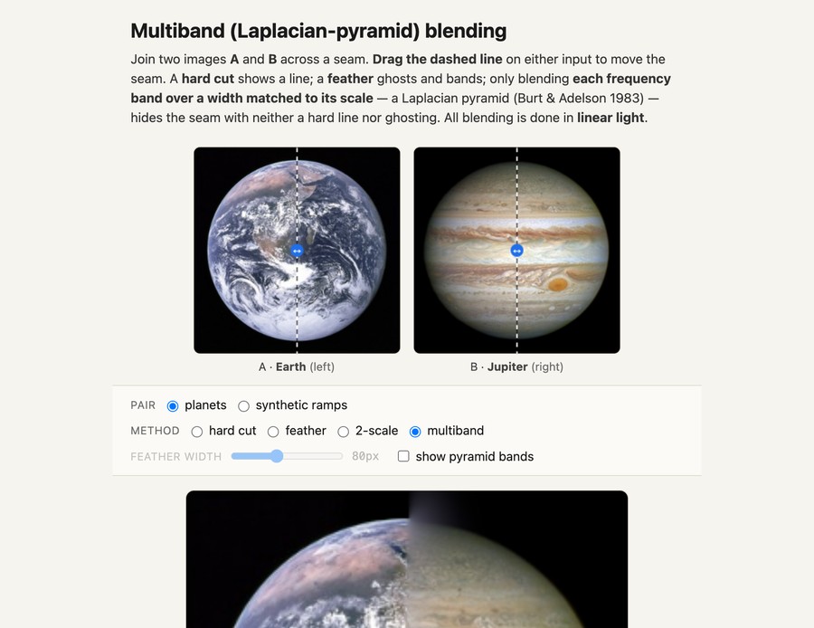
A Laplacian pyramid provides a finite set of scales, not a continuum. Burt and Adelson blend corresponding band-pass levels using masks whose support grows with scale (Burt & Adelson 1983 (Laplacian pyramid); Burt & Adelson 1983 (spline blending)). Include the coarsest residual and use matching expansion operators during reconstruction (Chapter 6.6, Pyramids and wavelets).
The per-band blend is one line. At each level $k$ take a convex combination governed by a mask $m^k$,
and reconstruct by collapsing, $I_{\text{out}} = \sum_k \operatorname{expand}(L^k_{\text{out}})$. The whole method is build-two-pyramids, blend-each-band, collapse:
LA = laplacian_pyramid(A)
LB = laplacian_pyramid(B)
GM = gaussian_pyramid(mask)        # mask blurred more at coarse levels
for each level k:
    L_out[k] = GM[k] · LA[k] + (1 - GM[k]) · LB[k]
return collapse(L_out)
Build the masks with a Gaussian pyramid so they remain smooth blending weights rather than signed band-pass coefficients. Fine-band transitions are narrow in source-image units; coarse transitions are wider. With several sources and incomplete coverage, normalize valid weights at each level. Extend source data and masks consistently to prevent invalid borders contaminating the pyramid.
Building the Gaussian and Laplacian pyramids correctly requires blurring before you decimate at every level. Skip the prefilter and high frequencies alias into the coarse levels, and once aliased, they masquerade as genuine low frequencies. The blend then produces bold false low-frequency artifacts (moiré, color blotches) that no amount of clever masking can remove, because the masking operates band-by-band and the corruption is in the wrong band. The pyramid's quality is only ever as good as its prefilter. This is why the pyramid construction, not merely the blend formula, is load-bearing here. (Big lesson L16; first appears in BASIC (Resampling). See Chapter 6.6, Pyramids and wavelets.)
Replace the spatial mask $m$ with a per-pixel quality weight (well-exposedness, local contrast, saturation) and the identical machinery fuses an exposure bracket straight into a tone-mapped image. That is exposure fusion (Mertens et al. (exposure fusion)), which ships on phones: same pyramid blend, different mask, no high-dynamic-range (HDR) radiance map ever formed. We return to it in the HDR and cell-phone chapters.
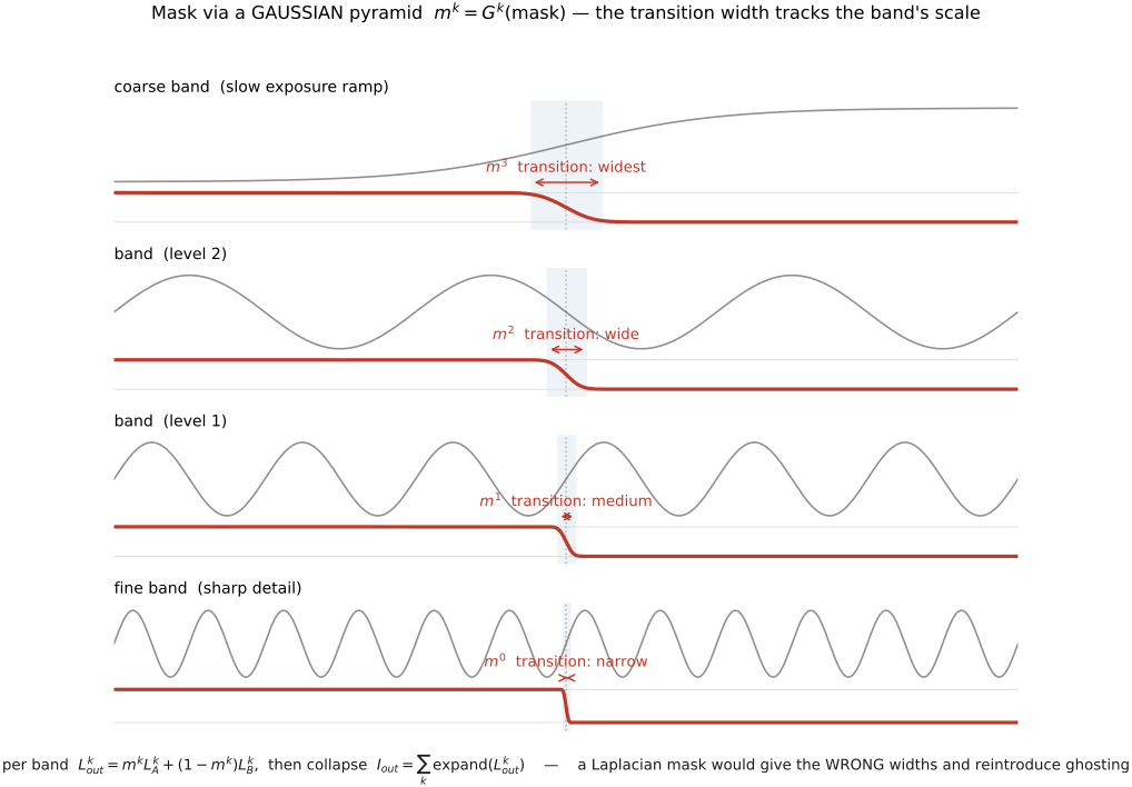
The image and mask pyramids have different jobs. The image's Laplacian bands separate detail by scale. The mask's Gaussian levels remain smoothly varying selection weights; they are not signed detail coefficients. At a coarse image level, a transition spanning a few samples covers a wide region in the original image. At a fine level, the transition covers fewer original pixels. Thus a broad exposure mismatch can blend gradually while fine texture changes source over a narrower region. This improves the compromise available to one fixed feather width, but it cannot repair geometric misalignment or guarantee an invisible seam.
20.3.5 Poisson / gradient-domain blending: paste gradients, solve for values⧉
The next rung changes the object of manipulation entirely. Instead of mixing pixel values across the seam, we mix the gradient field (Pérez et al. 2003). Inside the region being pasted, demand that the result's gradient match the source's gradient; on the boundary, demand that the result match the target's values; then solve for the pixels whose gradients best satisfy both. This is the same solve as seamless cloning (here the "source region" is one panorama image and the "background" is the other), and the worked single-image version, with its derivation, discretization, and solvers, is the subject of Chapter 10.8, Poisson image editing. We state the objective and read off the consequence; we do not re-derive.
The objective is a least-squares fit of the output's gradient to the prescribed guidance field $\mathbf{v}$ (the pasted source gradient), with the boundary pinned to the target:
Setting the derivative of that quadratic energy to zero gives its Euler–Lagrange condition, the Poisson equation $\nabla^2 f = \operatorname{div}\mathbf{v}$, a large sparse linear system, solved matrix-free with conjugate gradient (never forming the matrix, just repeated Laplacian convolutions), as worked out in Chapter 10.8, Poisson image editing.
The Dirichlet boundary fixes values, not their normal derivatives. The Poisson solve finds the closest feasible gradient field in the chosen norm; it does not force every gradient to match or guarantee an invisible seam. Boundary conditions can spread color changes throughout the pasted region.
Pyramid blending includes a coarse-scale mixture of the sources. Poisson blending instead uses the target boundary to anchor reconstructed values while fitting source gradients. That can change the source's overall tone and color. Compare the methods on flat regions as well as texture; neither guarantees the preferred brightness or correct scene lighting.
A linear-light Poisson solve preserves additive differences approximately, which can change relative contrast when the background level changes. A log or other perceptual-domain formulation changes the objective and requires careful handling of zeros and color. Mixed gradients choose a guidance derivative from source or target under a stated rule; they can preserve useful structure or introduce inconsistent texture (Chapter 10.8, Poisson image editing).
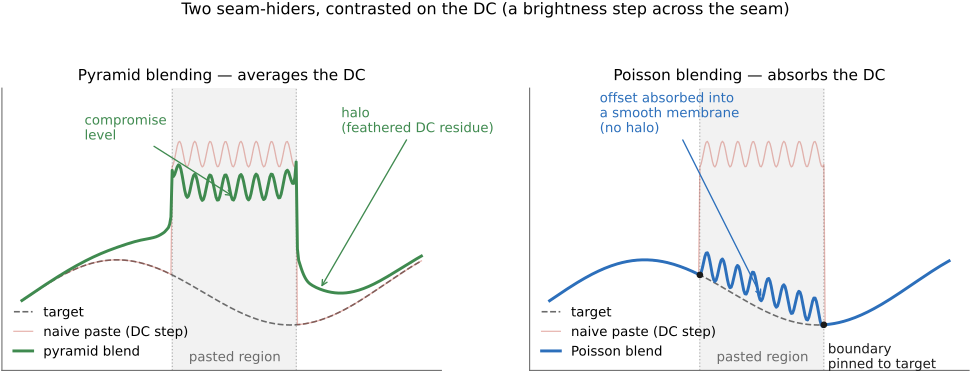
Try pasting a constant gray patch into a brighter constant background. The source has zero interior gradients. A Poisson reconstruction constrained by the target boundary can therefore fill the patch at the target level without violating those source gradients. Pyramid blending instead combines the coarse levels of both sources and can retain a gradual contribution from the darker patch. The difference is useful when choosing a method: a composite may benefit from shifting the pasted region's level, whereas a panorama may need explicit exposure calibration before any blend. Fitting gradients and mixing coarse intensities give different controls over that decision.
20.3.6 Seam optimization: route the seam instead of fading it⧉
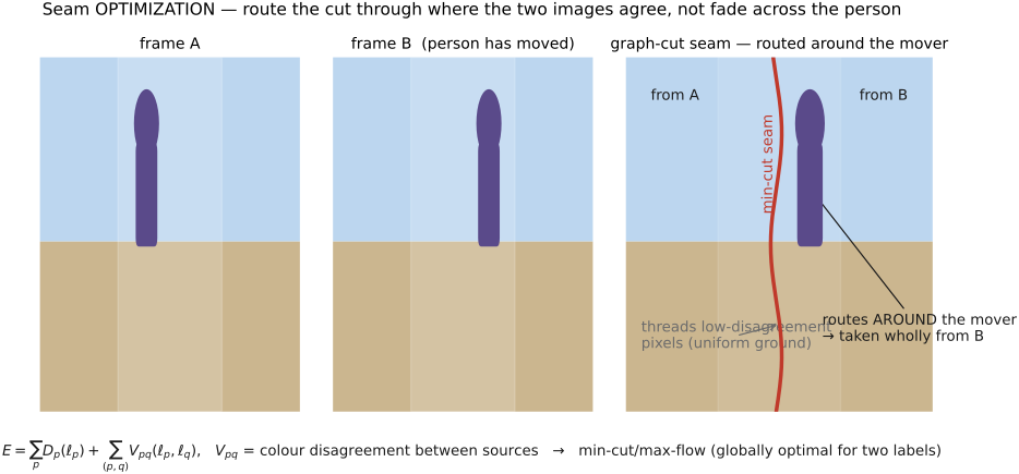
Every rung so far blends over a fixed seam, wherever the overlap happens to fall, and then works to disguise it. Seam optimization asks the prior question (Agarwala et al. 2004, Kwatra et al. 2003): where should the seam even be? Choose the boundary so it threads through pixels where the two images already agree, and there is barely anything left to blend. Route it along a uniform patch of sky rather than across a face, and the seam is half-hidden before any blending begins (Figure 20.3.8).
This is naturally posed as discrete optimization on a graph. Label each output pixel with the source it comes from, $\ell_p$, and minimize an energy with two terms,
a data term $D_p$ (a label must respect coverage: a pixel can only take a source that actually covers it) plus a smoothness term $V_{pq}$ that penalizes a label change between neighbors by how much the two sources disagree there. Minimizing $E$ over the two-source case is a min-cut / max-flow computation (a graph cut), which is globally optimal for a fixed binary submodular energy. Arbitrary two-label costs and general multi-label problems do not share that guarantee. The mechanics are the subject of Chapter 10.9, Seam optimization.
The optimizer here is standard: graph cut / min-cut is a solved problem. The energy is the entire design. Set $V_{pq}$ to the color disagreement between the sources at this edge, and the min-cut automatically prefers to cut where the images match, along a uniform sky, not through a person's face. This is the affinity principle turned inside out: instead of "average things that belong together," it is "do not cut between things that belong together." The art is choosing what counts as disagreement, not running the solver. (Big lesson L10.5; first appears in Chapter 10.9, Seam optimization.)
How does this compose with the rest of the ladder? Seam optimization decides where to put the boundary; you then still run a Poisson or pyramid blend across that optimal seam to mop up whatever residual exposure mismatch survives. Graph-cut then gradient-domain reconstruction is the canonical photomontage recipe (Agarwala et al. 2004): cut along the edges, then reconstruct across them. It is the explicit meeting point of this part's blend ladder with the gradient-domain leg of EDGES MATTER.
Motion-aware seam costs or explicit region constraints can favor taking an object from one frame. Color disagreement alone does not guarantee that the whole object receives one label; missing background coverage can also prevent removing it.
20.3.7 The complete pipeline, end to end⧉
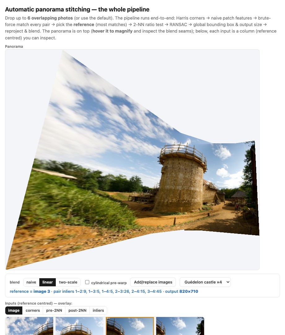
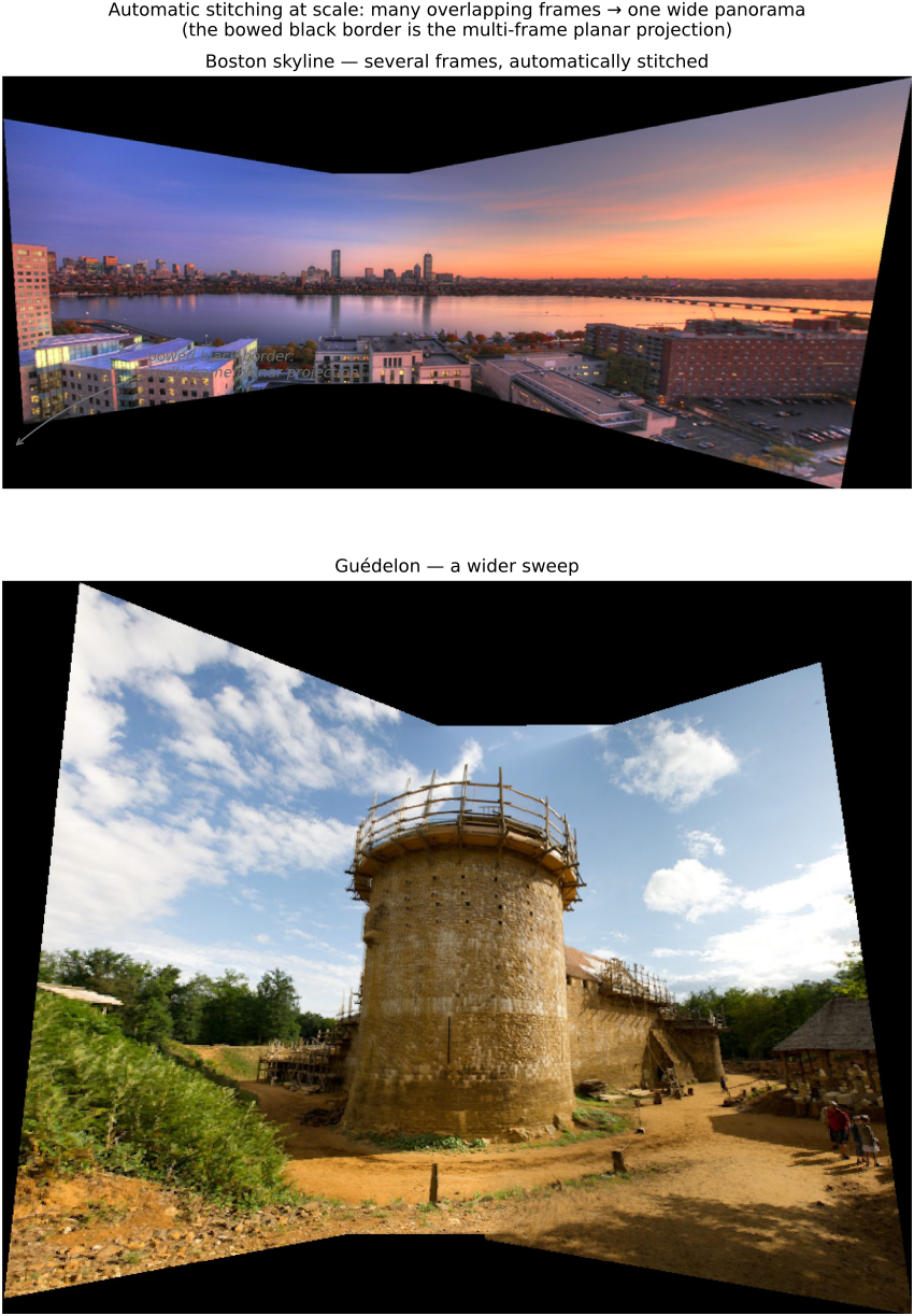
With blending built up (from the hard seam through feathering, two-scale, multiband, Poisson, and seam routing), the panorama pipeline is finally complete. We can now put the whole thing in one place: the geometry of Chapter 20.2, Automatic panorama stitching from multiple views and feature matching (detect → describe → match → RANSAC → warp) followed by the photometric step of this chapter (blend). The interactive stitcher below runs every stage live, and the gallery shows the same pipeline scaled to many hand-held frames, both deferred here from the matching chapter precisely because the final blend they depend on is only now in hand.
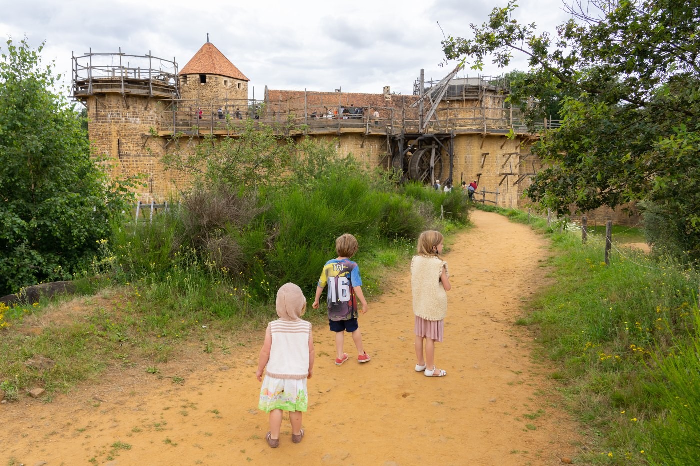
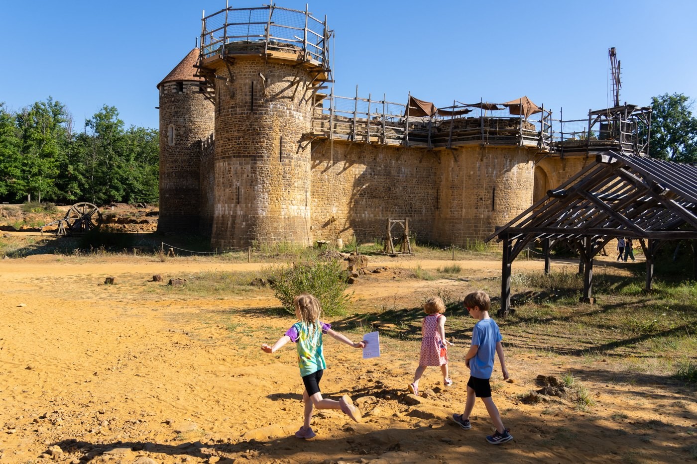 The default scene in the stitcher below, and the panorama in the gallery, is Guédelon, a medieval castle in Treigny, Burgundy, France, that since 1997 has been built from nothing using only 13th-century methods and materials: stone quarried on site, oak hewn with period tools, lime mortar burnt in wood-fired kilns, a human-powered treadwheel crane. It is experimental archaeology run as a decades-long public project, and the walls rise a little each year. These photographs are the (human) author's own: Guédelon sits about ten miles from where Frédo grew up, which is why it shows up here as a test scene rather than a laboratory scene. The overlapping, slightly exposure-varied frames of its big round tower make it a good blending workout.
For a multi-image panorama, refine geometry and photometry over the overlap graph, then resample the original frames into the chosen output projection (Chapter 20.4, Bells and whistles). Blending operates on those sources and validity masks.
Recap: big lessons of this chapter
A source change can introduce an edge that was absent from the scene. Blending reduces that discontinuity or moves the transition to a less conspicuous location. Smooth brightness and color errors can remain visible, so inspect the whole image as well as the seam.