20.2 Automatic panorama stitching from multiple views and feature matching⧉
PS7 builds the automatic panorama: Harris, descriptors, the 2NN test, RANSAC, and blending. → Chapter 1.5, Problem sets (appendix).
The manual stitcher needs corresponding scene points. Automatic feature matching supplies candidates, then geometric estimation tests which can be explained by a common map. Preserve that verification step even when a descriptor match looks confident.
A wide panorama requires enough overlap and distinctive content to connect the images. Repeated windows, blank walls and moving subjects can defeat an otherwise appropriate estimator.
The same pipeline runs in many places: phone panorama modes, 360° cameras that stitch several fisheye views, robotic heads that shoot gigapixel mosaics tile by tile, aerial and satellite mosaics, and whole-slide scanners in microscopy. In the book's terms a panorama is multiple-exposure imaging along the field-of-view axis, as a bracket extends range and a focal stack extends depth of field; varying position rather than direction leads instead to light fields and 3-D reconstruction, where one homography no longer explains the images.
20.2.1 Why not brute force, and the two sub-problems⧉
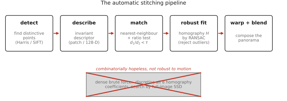
Exhaustively sampling eight homography coefficients is impractical. Sparse features provide an initialization from selected points. Direct alignment is another useful method: with a good initialization, iterative image-based optimization can estimate or refine a transform without an exhaustive search (Chapter 12.1, Brute force).
Interest points concentrate the match search on localized structure. Flat regions offer little local position information, while edges constrain motion mostly across the edge. Feature matching can still fail on repeated patterns or large appearance changes.
That plan decomposes into two sub-problems, the chapter's skeleton:
- repeatable detection: detect the same scene point independently in each image. If a point is found in one image but missed in the other, it can never be matched, no matter how good the rest of the pipeline is. Detection must therefore be repeatable across the changes of viewpoint, scale, and lighting that separate two frames.
- distinctive description: for a detected point, summarize its neighborhood with a descriptor that is similar for the same scene point seen in two views and different for unrelated points, so that the correct correspondent can be recognized among many candidates.
In a classical detector/descriptor pipeline, features are computed independently and then matched. Joint learned matchers can exchange information between images, so independence is a property of this baseline, not a rule for every algorithm.
20.2.2 The feature pipeline, recalled⧉
The detect → describe → match → robustly-fit pipeline is built in full in Part 12, Matching pixels across space and time, and there is no profit in re-deriving it here. Chapter 12.3, Sparse matching, develops the detectors and descriptors: the structure tensor $M=\sum w\,\nabla I\,\nabla I^\top$ and its eigenvalue partition into flat / edge / corner, the Harris response $R=\det M-k(\operatorname{tr}M)^2$ and Shi–Tomasi, the scale axis that Harris lacks, and SIFT: Difference-of-Gaussians scale-space, the 26-neighbor space-and-scale extremum, a canonical orientation, and the $4\times4\times8=128$-dimensional descriptor, together with the broader detector/descriptor zoo. Chapter 12.5, Robustness: the ratio test and RANSAC, develops the clean-up: Lowe's ratio test and RANSAC. For panorama stitching we simply use that pipeline, so a one-paragraph recall is enough before we turn to the homography-specific orchestration that this chapter owns.
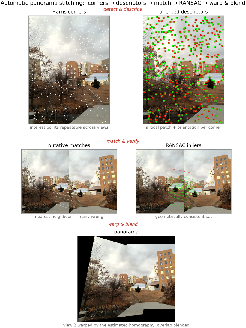
Here is the pipeline as it runs on a pair of overlapping frames, with each stage a pointer into that part (Figure 20.2.1):
- Detect distinctive points independently in each image: Harris corners, or SIFT keypoints when scale and rotation invariance are needed (Chapter 12.3, Sparse matching). Detection is run separately per image and must be repeatable: a point found in one view but missed in the other can never be matched.
- Describe each point's neighborhood with an invariant vector $\mathbf{f}$: a normalized patch, or the 128-D SIFT descriptor (Chapter 12.3, Sparse matching). The descriptor must be distinctive yet invariant: similar for the same scene point across the two views, different for unrelated points.
- Match by nearest descriptor, then prune the ambiguous matches with Lowe's ratio test $d_1/d_2<\rho$ (with $\rho\approx0.7$–$0.8$, the threshold called $\rho$ in Chapter 12.5, Robustness: the ratio test and RANSAC), which keeps a match only when its nearest descriptor is decisively closer than its second-nearest. This raises the inlier fraction $w$ that RANSAC will exploit next.
- Robustly fit the model, here the homography $H$, from the surviving, still-outlier-ridden matches with RANSAC (Chapter 12.5, Robustness: the ratio test and RANSAC). The remainder of this chapter is about what "for us" means: how RANSAC specializes to a homography.
After feature initialization, direct photometric refinement can use additional image information when exposure and visibility are modeled appropriately.
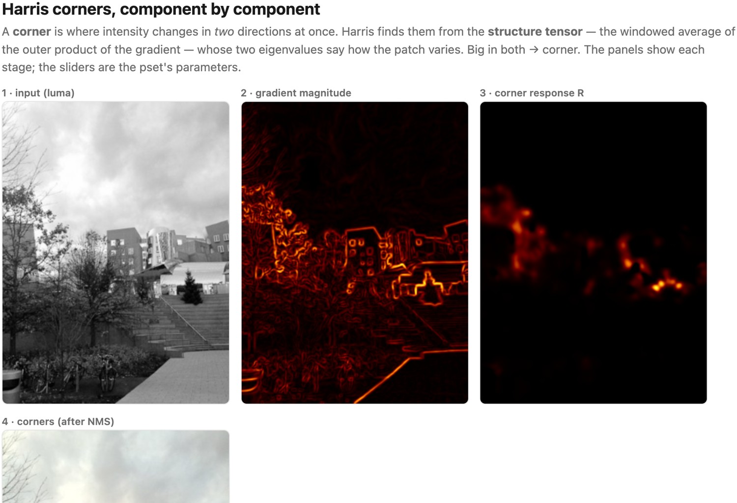
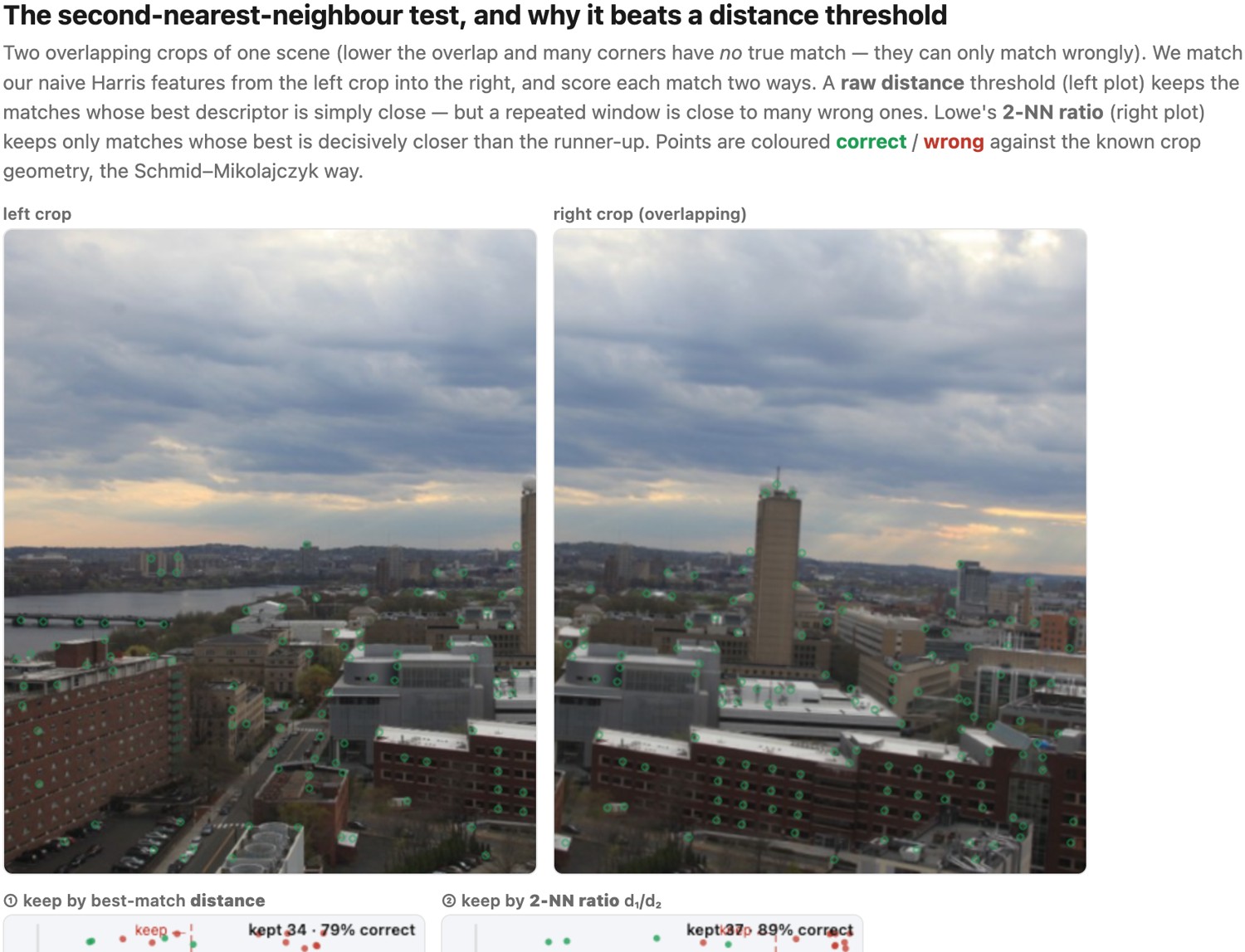
A synthetic warp provides exact correspondence truth but omits many real capture changes. Evaluate ratio and distance thresholds on repeated texture, exposure differences and non-overlap. The ratio test rejects ambiguity in descriptor space; it can also reject correct matches or retain a wrong distinctive one.
20.2.3 RANSAC for a homography⧉
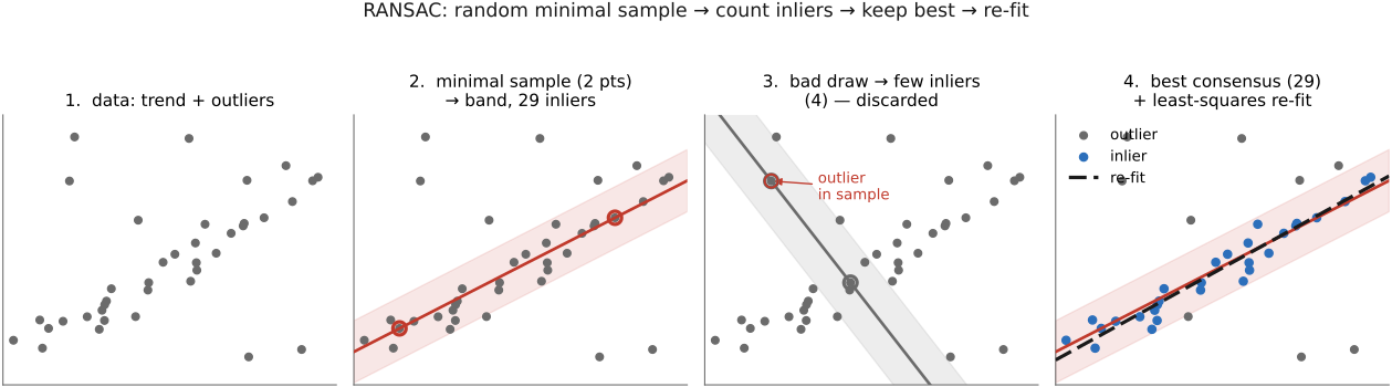
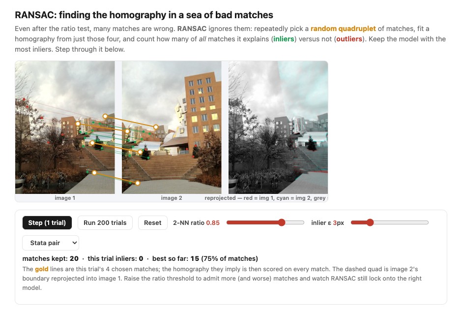
We now have point correspondences, most of them good (inliers) but some still wrong (outliers), and we want the homography $H$. A plain least-squares fit over all matches is hopeless: least squares minimizes squared error, which gives large residuals disproportionate influence, so even a handful of gross outliers drags the fit arbitrarily far from the truth. We need a robust estimator, one that can find the right model while ignoring the bad data.
RANSAC, RANdom SAmple Consensus, due to Fischler and Bolles (1981), does this with a simple loop:
Project homogeneous coordinates before measuring pixel error. Define $\pi(a,b,c)=(a/c,b/c)$ and use
where $\tilde{\mathbf x}_i$ is the homogeneous source point and $\mathbf x_i'$ is the two-dimensional target. Reject unstable denominators. A symmetric transfer error can additionally measure the reverse direction.
best_inliers = []
for trial in range(iteration_budget):
    sample = random_distinct_matches(4)
    if degenerate(sample): continue
    H = normalized_DLT(sample)
    if invalid_model(H): continue
    errors = projected_pixel_errors(H, matches)
    inliers = indices_where(errors < tolerance_pixels)
    if better_consensus(inliers, errors, best_inliers):
        best_inliers = inliers
if len(best_inliers) < 4:
    return failure("insufficient consistent matches")
H = normalized_DLT(matches[best_inliers])
H = refine_geometric_error(H, matches[best_inliers])
return validate_and_rescore(H, matches)
Choose the tolerance in the coordinates actually scored; resizing changes pixel units. Check spatial coverage as well as the number of inliers. A large cluster on one repeated facade can support an incorrect or poorly extrapolated panorama.
RANSAC searches for a model supported by many correspondences. An all-inlier minimal sample can still be poorly conditioned, and repeated structure can support a coherent wrong model. Sampling, scoring, refitting and final validation are all needed.
Under independent trials with inlier fraction $w$ and minimal sample size $s$, a conventional budget is
For $w=0.5$, $s=4$ and $p=0.99$, this gives 72 draws. It estimates the chance of at least one all-inlier sample, not the probability of a correct final panorama. Degeneracy, correlated matches and an inaccurate inlier estimate weaken that interpretation. Bound the budget and handle $w=0$ and $w=1$ explicitly (Chapter 12.5, Robustness: the ratio test and RANSAC).
The two-image pipeline now estimates a map from automatic matches. Multi-image systems also need a reliable overlap graph, globally consistent camera estimates and photometric compensation; Brown and Lowe combine these with blending (Brown & Lowe 2007). Disconnected groups should produce separate panoramas or a clear failure, not an arbitrary placement.
Match reliable overlapping pairs and retain the original frames. Use the overlap graph to initialize camera poses, then refine globally (Chapter 20.4, Bells and whistles). Repeatedly resampling a growing mosaic can accumulate blur; render original sources into the final canvas once.
There is one stage we have black-boxed throughout as "warp and blend": the final compositing of the overlapping, exposure-mismatched frames into a seam-free image. It is substantial enough to own the next chapter, and it is the last thing standing between this pipeline and a finished panorama. So the complete end-to-end interactive stitcher, and a gallery of many-frame results, are deferred to the end of Chapter 20.3, Blending, once the blend step they depend on has actually been built, where you can run detect → describe → match → RANSAC → warp → blend in one place. See "the complete pipeline, end to end" there.
The panorama merge of Chapter 8.13, A raw developer in the browser is this pipeline end to end, with the analysis view showing corners, accepted and rejected matches, and the bundle adjustment's before/after; the result installs as a re-editable photograph.
An incorrect match can have a very large residual under the correct homography, so including every match in ordinary least squares lets a few bad pairs pull the fit away from the true alignment. RANSAC temporarily fits a small subset and asks how many other pairs support that geometric explanation. The minimal subset itself is not the final estimate: after finding a useful consensus, refit using its inliers and check their residuals and spatial distribution. Four nearly collinear pairs, or many inliers clustered in a small corner, constrain the geometry less reliably than well-distributed correspondences.
The exponent $s$ explains why RANSAC draws a minimal sample first and uses more points only after finding consensus. At $w=1/2$, a four-point sample is all-inlier with probability $1/16$; an eight-point sample has probability $1/256$. Adding points to each random hypothesis can therefore make finding a clean one much more expensive. A matching filter helps when it raises the inlier fraction while retaining enough well-distributed correct pairs; discarding matches indiscriminately does not guarantee that improvement.