19.1 Transparency and compositing🔗⧉

A cutout can have the right silhouette and still acquire a dark fringe when resized. Compositing depends on both the matte and the representation of its color. Establish that representation before filtering, stacking layers or replacing a background.

Layers make this the forward direction of a larger problem: given colors and coverage, form a picture. Segmentation and matting work backward from a picture to isolate its subjects. Keeping that distinction in mind explains why compositing can be a short equation while extracting the quantities it needs is an ill-posed inference problem.

19.1.1 Compositing and alpha channels🔗⧉

Before we can pull a subject out, we should be precise about what it would mean to lay one back down. The model is the compositing equation, put on a firm digital footing by Porter and Duff (Porter and Duff 1984, "Compositing Digital Images", the paper that gave us the alpha channel as we use it). A foreground element carries, besides its color $F$, a fourth channel $\alpha$, and dropping it over a background $B$ is the per-pixel over operator

For an opaque edge, alpha can represent fractional pixel coverage. For neutral attenuation it can represent opacity. These interpretations share a useful approximation, but a single scalar does not describe arbitrary colored transmission, refraction or correlations between subpixel foreground and background structure. Composite in a common linear-light color space when the goal is light mixing.

Premultiplied (associated) alpha. There is one subtlety in how $F$ and $\alpha$ are stored together, and it is the source of more haloed composites than any other single mistake. In straight (unassociated) alpha, you store the foreground's true color $F$ and its coverage $\alpha$ separately. In premultiplied (associated) alpha, you store the color already scaled by coverage, $F' = \alpha F$, alongside $\alpha$. The over operator then reads

Filter associated color and alpha with the same linear operator. Hidden RGB under transparent pixels then contributes zero; ordinary independent filtering of straight RGB and alpha can leak that hidden color into visible edges. Straight-alpha storage is valid, but resampling must account for coverage. Unpremultiply only when needed and guard small alpha.

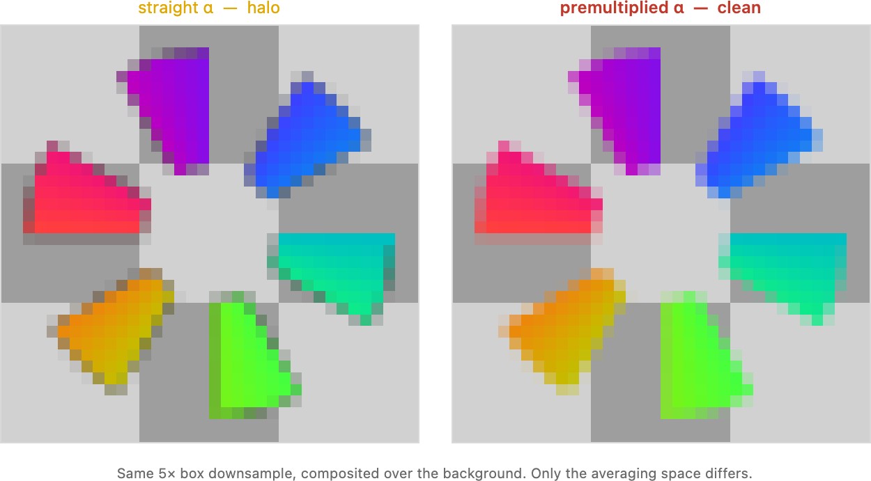
Carrying weighted color and weight together also appears in normalized filtering (Chapter 10.1, Bilateral filtering). The algebra resembles homogeneous coordinates, but alpha has a coverage or opacity interpretation and is not a projective coordinate. Premultiplication prevents hidden RGB in transparent pixels from contaminating ordinary resampling.

For two partially transparent layers, store associated colors $c_A=\alpha_A F_A$ and $c_B=\alpha_B F_B$. Their over composite is

The background's alpha is part of the calculation. Over is associative in this representation, but not commutative: grouping layers preserves the result while changing their order generally does not. Unpremultiply only when needed, guarding zero or very small alpha.

linear_rgb = decode_color(straight_rgb)
associated = alpha * linear_rgb
associated = resample(associated)
alpha = resample(alpha)              # same geometry, kernel and boundary convention
result = associated + (1-alpha) * background_linear

Alpha is a linear coverage/opacity quantity; do not apply an RGB transfer function to it. Negative-lobe resampling kernels can overshoot alpha or associated color, requiring a deliberate policy. Nonlinear color edits may require unpremultiplication and subsequent reassociation.

Layers retain editable colors, alpha and ordering. Blend modes modify the color-combination rule in a declared working space; for opaque inputs, multiply uses $F B$ and screen uses $1-(1-F)(1-B)$. With partial transparency, the blend function and alpha compositing must both be applied consistently. Save a format that preserves the needed layers and alpha; a standard JPEG flattens the result.

Chapter 19.2, Segmentation identifies regions or objects. Chapter 19.4, Matting estimates the fractional mixture near boundaries and within translucent structure. A soft segmentation confidence is not automatically the physical alpha required by the compositing equation.

A two-pixel example explains why filtering straight RGB and alpha independently can make a fringe. Let one pixel be opaque red and its neighbor fully transparent with an arbitrary blue RGB value. Their straight-RGB average is purple and their average alpha is one half. Compositing that result over black contributes both red and blue, even though the blue pixel was completely invisible. In premultiplied storage the transparent pixel has zero weighted color. Averaging instead gives half red with alpha one half, which composites without the blue fringe. The arbitrary RGB stored behind zero alpha never enters the result.

This resembles accumulating weighted colors and weights during blending, but premultiplied alpha also has a specific compositing interpretation. Do not divide a premultiplied image by alpha before every filter; keep the weighted representation through operations that expect it, and define the zero-alpha case when unpremultiplication is needed.

The bookkeeping can be compared explicitly with normalized filtering. A weighted average carries $(\sum_i w_i c_i,\sum_i w_i)$ through accumulation and divides only afterward. A premultiplied color carries $(\alpha R,\alpha G,\alpha B,\alpha)$ through filtering. If a fully transparent texel has an arbitrary RGB value, multiplying by its zero alpha prevents that hidden color from leaking into its visible neighbors during interpolation. Storing the weight beside the weighted quantity also resembles $(wx,wy,w)$ in homogeneous coordinates, although alpha denotes coverage or opacity rather than a projective scale. The shared computational idea is to postpone division while combining the weighted quantities.

19.1.2 Harmonization and where the blends live🔗⧉

Suppose the cut is finally perfect, a flawless soft $\alpha$, every wisp of hair accounted for. Drop the cutout onto the new background and it can still look wrong: it sits there "stickered on," lit by a different sun, white-balanced by a different camera, carrying a different contrast and grain than its new surroundings (Figure 19.1.2⛶ fullscreen). The matte was right; the appearance is wrong. Fixing that takes two further layers, both built in EDGES MATTER and only invoked here.

Poisson blending adjusts colors to approximate a chosen gradient field subject to background boundaries (Chapter 10.8, Poisson image editing). Pyramid blending mixes frequency bands (Chapter 20.3, Blending). Neither guarantees correct illumination, contact shadows or reflection. Color-statistics transfer (Reinhard et al. 2001) addresses some appearance differences; changing illumination direction may require relighting and geometry, beyond a global color adjustment.

Interactive digital photomontage selects source regions with graph cuts and blends their boundaries (Agarwala et al. 2004). It shares selection and blending tools with compositing, while HDR merging combines calibrated observations for a different purpose (Chapter 17.3, Merging exposures).

A group portrait gives a concrete example of photomontage: choose one person's smile from one frame and another person's open eyes from another. Source selection decides whose pixels to use; blending handles the joins. Neither decision is the radiometric weighting of an HDR merge. Likewise, a face lit from the left can retain contradictory shading when placed in a scene lit from the right, even after its boundary colors have been adjusted. Matching the seam and matching the illumination are different tasks.

19.1.3 Optical effects beyond alpha🔗⧉

Everything in this chapter rests on one model of a foreground pixel: $C=\alpha F+(1-\alpha)B$, the object partially covers the background, and a single number $\alpha$ says how much. That is exactly right for an opaque object with a soft, anti-aliased, or wispy edge. But a great many real foregrounds do not merely cover the background: they refract, reflect, attenuate, and scatter it. Look through a wine glass, a water droplet, a magnifying lens, a sheet of frosted glass, or a strand of fiber-optic: the color you see at a pixel does not come from the single background point directly behind it, but from some other region of the environment that the object bent the light from, and often from several regions at once, tinted and blurred. No alpha, however soft, can express "this pixel shows you what is 30° to the left, flipped and colored green." The linear coverage model simply has no slot for it.

Environment matting (Zongker, Werner, Curless & Salesin 1999) generalizes the matte to capture exactly this. Instead of one $\alpha$ per pixel, it records, for each foreground pixel, which parts of the surrounding environment contribute to it and how, effectively a small light-transport descriptor per pixel (a region of the background, plus reflectance/attenuation and color), measured by photographing the object in front of a sequence of structured backdrops (Gray-coded stripes), the same swept-pattern trick as structured light and the transport-matrix capture of dual photography (Chapter 35.4, Separation of direct and global illumination and dual photography in Part 35, Computational illumination). With that descriptor in hand you can re-composite a refractive or specular object over a brand-new background and have it convincingly distort, mirror, and tint that scene, a glass that actually refracts whatever you place behind it. Chuang et al. (2000) pushed it to higher accuracy and toward real-time and video capture.

Environment matting estimates how an object redirects light under a capture model. The measured transport is tied to its geometry and acquisition setup; it is not an unrestricted replacement for relighting or rendering a new viewpoint.

This changes what it means to extract an object. An ordinary matte records where a foreground contributes. An environment matte additionally records how the object transports light from its surroundings. That shift connects compositing to the measurement of light transport in Part 35, Computational illumination.