18.7 Tone mapping as perceptual optimization⧉
The operators of the previous chapters choose a functional form, a sigmoid, a compressed base, an attenuated gradient, and tune its parameters by eye. A different paradigm starts from the other end: write down a model of the viewer's vision and of the display, define how far the displayed image is from the scene in terms of that model, and solve for the rendering that minimizes it. The tone curve is then an output, not a choice. This is the most direct answer to the question "what should the curve be", and it fits the appearance goal of Part 18, Tone mapping and display best. This chapter presents the two main representatives, one built on contrast visibility and one on color appearance, and explains why neither displaced the simpler methods in practice.
18.7.1 Display-adaptive tone mapping⧉
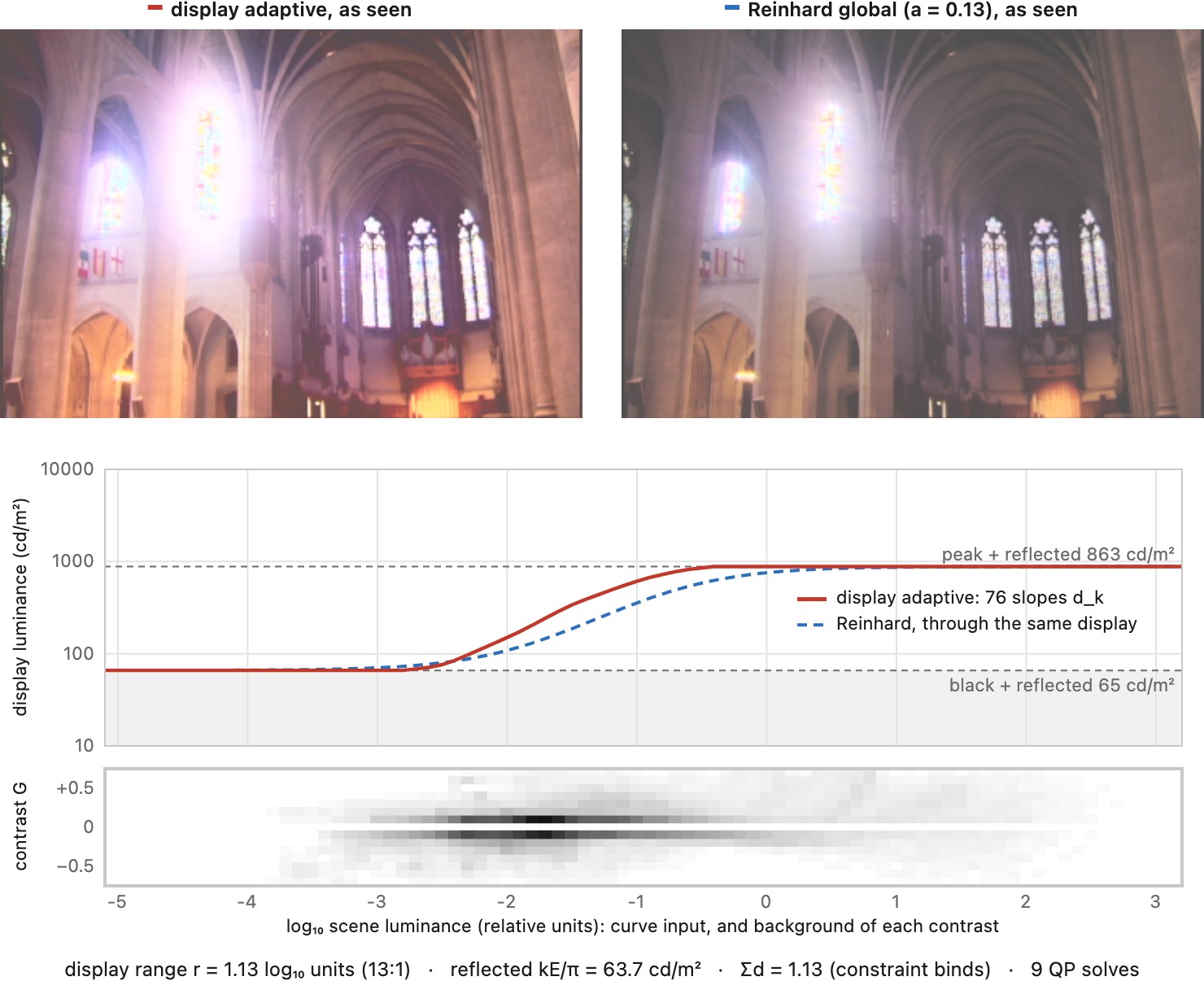
Mantiuk, Daly and Kerofsky pose tone mapping as an optimization with two explicit models Mantiuk, Daly & Kerofsky 2008. The display model gives the luminance a pixel value produces, including the display's peak, its black level and the ambient light reflected from its surface, so the same curve is evaluated differently in a dark room and in daylight. The visual model converts luminance contrast into a perceived response, through a contrast transducer derived from contrast-discrimination data at the relevant adaptation level, so that a contrast below threshold counts for nothing and a large contrast is compressed in perception as it is in vision.
The objective compares, for every contrast that occurs in the image, the visual response it produced in the scene with the response it produces on the display, and sums the squared differences, weighted by how often each contrast occurs at each luminance, a statistic computed from the image itself. The unknown is a tone curve, represented as a piecewise-linear function of log luminance with one slope per segment. The constraints say that the curve is monotonic and that its output stays within the display's range. Because the transducer is applied to the curve's slopes, the problem is a quadratic program and solves quickly.
The resulting curve spends the display's contrast where the image has contrasts that would otherwise become invisible, and compresses ranges where the image has little. It is related to earlier operators: weighting by how often contrasts occur gives it the adaptivity of histogram equalization, and the transducer, which counts invisible differences as nothing, plays the role of the visibility bound in Ward's histogram adjustment (Chapter 18.2, Global tone mapping). What is new is the display. When the ambient light rises, the curve lifts the shadows, giving the darkest tones higher code values so that they stay distinguishable once the room's reflected light is added; measured in displayed luminance, their contrast still falls, since the reflections dominate there. When the display's peak drops, the curve compresses the highlights harder, and in daylight it clips the sparsest highlights, a few percent of the pixels, to keep contrast where the image has more of it. In a dark room the optimized rendering can look darker than Reinhard's. The same radiance map gets a different rendering for each display and room, which is the right behavior and one no hand-tuned curve has.
Figure 18.7.1 solves this program for one radiance map and for a display and room the reader chooses.
18.7.2 iCAM06: the color appearance route⧉
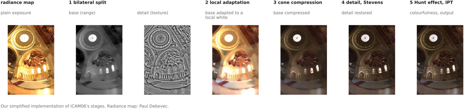
Kuang, Johnson and Fairchild approached the same problem from color appearance modeling Kuang, Johnson & Fairchild 2007 (iCAM06). Their image appearance model iCAM06 applies to an image the components that color appearance models such as CIECAM02 apply to uniform patches (Chapter 4.5, Advanced color: opponents, perceptually-uniform, and preferred). It splits the image into a base and a detail layer with a bilateral filter, as in Chapter 18.3, Two-scale and bilateral tone mapping. On the base it performs chromatic adaptation to a local white point, taken from a blurred version of the image, and compresses the range with a model of cone and rod responses. It then restores the detail with a gain that follows the Stevens effect, adjusts colorfulness for the Hunt effect, and converts the result to the display through the inverse model (Chapter 18.1, Tone mapping and perception). Each step is a measured property of vision rather than a parameter chosen by eye, and the output aims at the appearance an observer would have had in the scene.
Figure 18.7.2 runs the stages on one radiance map.
18.7.3 Why they did not take over⧉
Neither approach displaced the simpler operators of the earlier chapters, for reasons that say more about the problem than about the methods.
Both need information that is usually missing. A visual model needs the scene's absolute luminance, in candelas per square meter, and the display's peak, black level and ambient light. Most radiance maps are only relative (Chapter 17.2, Camera response and radiance calibration), and most pictures are seen on displays and in rooms nobody measured. With guessed inputs, the advantage of a principled model shrinks.
They optimize the second goal, and most products want the third. Display-adaptive tone mapping minimizes visible contrast distortion, and iCAM06 reproduces appearance; a camera or an editor is judged on whether people like the picture, and the preferred rendering often departs from the faithful one in ways the models count as errors (Part 18, Tone mapping and display).
They are harder to steer. Their parameters have physical meaning but no direct photographic meaning: a photographer who wants brighter shadows can move a curve, but not easily an adaptation model. And display-adaptive tone mapping is a global curve, with the limits of every global curve (Chapter 18.2, Global tone mapping).
Their ideas survived in other places. Display adaptation became central with HDR displays, whose range varies from one device to the next and whose rendering is adjusted to the display's peak and the room's light (Chapter 18.10, HDR displays and display mapping); the Stevens and Hunt compensations are now written into standards such as BT.2100; and the visual models became evaluation metrics, HDR-VDP among them (Chapter 18.11, Evaluating tone mapping).