18.1 Tone mapping and perception⧉
Camera pipelines already apply a tone curve to every photograph, the beauty curve, an S-shaped curve that lifts midtone contrast so that scene-linear values look right on a screen (Why scene-linear looks dull). This chapter puts perception science behind a large part of that craft: the midtone contrast above one, the toe that compensates for flare, and the extra colorfulness all follow from how a picture is seen (Perceptual basis for beauty curves). Not all of it: the softness of the shoulder, where middle gray sits and the colors a manufacturer prefers are matters of taste, which the end of the chapter separates from the perception.
A photograph is seen under conditions that have little to do with the scene it shows. The scene was lit by the sun at tens of thousands of candelas per square meter, filled the visual field, and was seen by an eye adapted to it. The print hangs under room light at a few hundred, the screen emits a few hundred to a thousand, both occupy part of the visual field, and both sit in a room that adds its own light. Appearance reproduction, the second goal of Part 18, Tone mapping and display, has to account for those differences. This chapter collects what it needs from the perception chapters (Chapter 3.3, Adaptation and constancy, Chapter 3.4, Spatial and temporal vision): four reasons a reproduction needs more contrast than the scene, and the spatial properties of vision that local tone mapping relies on.
The overall effect is usually summarized by an end-to-end, or system, gamma: the slope, in log-log coordinates, of the curve from scene luminance to displayed luminance in the middle tones. A system gamma of one reproduces the scene's ratios exactly. Every reproduction medium that looks right uses a system gamma above one.
This is a different quantity from the gamma of an encoding (Chapter 4.3, Encoding: linear, gamma or log). An encoding gamma is undone by the matching decoding: it changes the numbers that store the image, to spend code values where the eye needs them, but not the light that reaches the viewer. The system gamma is what remains of the whole chain once every encoding has been undone, and it changes the picture on purpose, to account for the viewing conditions (System gamma: the end-to-end curve, which also explains how the CRT supplied the decoding and the system gamma at once).
18.1.1 Why a faithful copy looks flat: four causes⧉
The effects below are each well documented; grouping them as four is our organization of Hunt's material on tone and color reproduction Hunt, The Reproduction of Color. The first three act on the luminance curve, the fourth on chroma.
Surround. An image seen against a dark or dim surround appears lower in contrast than the same image in an average surround, because the surround sets the reference for adaptation, and in darkness the picture's own dark tones read as relatively lighter. Bartleson and Breneman measured the effect in 1967 with complex images rather than isolated patches, which is why it transfers to pictures Bartleson & Breneman 1967 (surround). The working values of the compensating system gamma are about 1.5 for a dark surround, as in a cinema, about 1.25 for a dim one, as for television in a living room, and 1.0 for an average surround, such as a print viewed under the same light as its surroundings. The CIECAM02 color appearance model carries the same effect in its surround parameter $c$, set to 0.69, 0.59 and 0.525 for average, dim and dark surrounds (Chapter 4.5, Advanced color: opponents, perceptually-uniform, and preferred).
Absolute luminance: the Stevens effect. Perceived brightness contrast rises with the adapting luminance Stevens & Stevens 1963 (Stevens effect). A print at a few hundred cd/m², or a display at 100 to 1,000, reproduces a scene that was at 10,000 or more, so the reproduction looks flatter even with its ratios preserved, and its gamma must rise to compensate. This effect is now standardized rather than only described. ITU-R BT.2100 gives the system gamma of hybrid log-gamma video as a function of the display's peak luminance $L_W$,
which is 1.2 at 1,000 cd/m², about 1.03 at 400 and about 1.33 at 2,000: the rendering gets steeper as the display gets brighter. The formula is meant for HDR displays; it falls below one under about 330 cd/m², to 0.78 at 100, so it does not describe standard-range viewing (ITU-R BT.2100). A broadcast standard with a closed-form Stevens compensation is about as explicit as the field gets that this part of tone reproduction is perception rather than taste.
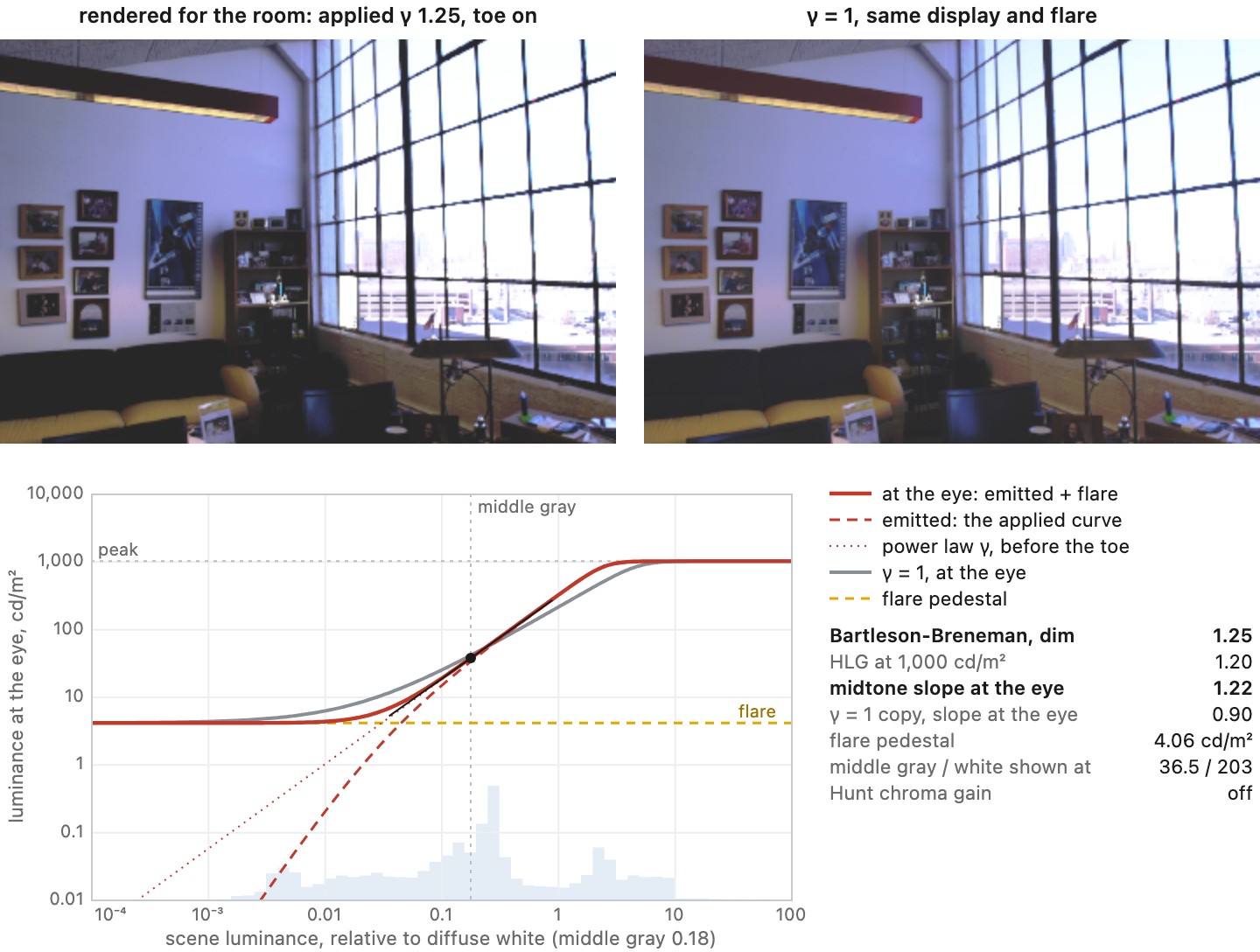
Flare. Veiling glare, in the camera and in the viewing environment, adds a roughly uniform pedestal of light in linear terms. Because it is added, its relative effect is largest in the darkest tones: a flare of 1% of white doubles a tone that was at 1% and leaves a midtone almost untouched, so it compresses shadow contrast specifically rather than uniformly. A few percent of peak white in a lit room removes the bottom two stops. In the simulator below, a flare of 1%, 2% and 5% of white lowers the midtone slope by about 5%, 10% and 22% when nothing compensates, and a toe brings the loss back to about 1%, 2% and 10%. The toe of a tone curve partly compensates for this, which means that part of what reads as an aesthetic crushing of blacks is recovering contrast that flare removed. It is also why the right rendering depends on the room, and why a cinema, a living room and an office want different curves (Chapter 18.10, HDR displays and display mapping).
Colorfulness: the Hunt effect. Colorfulness increases with luminance, so a reproduction at a fraction of the scene's luminance looks duller even when its chromaticities are exact Hunt 1952 (Hunt effect). Restoring the appearance requires a chroma boost whose size can in principle be derived from the luminance ratio. This is the one place where appearance reproduction licenses an increase in saturation, and consumer image pipelines push far beyond what it justifies; the excess is a preference for memory colors, not a restoration of appearance (Chapter 8.6, Color beautification and preferred colors).
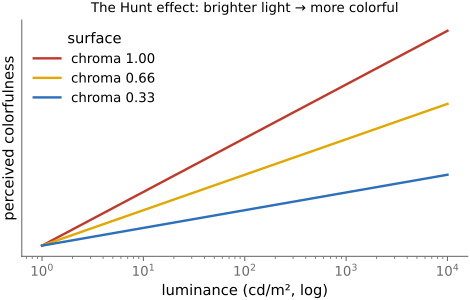
Figure 18.1.1 puts the four causes on one radiance map: the surround or the display's peak sets the applied gamma, the room adds its flare, and a toggle restores chroma for the Hunt effect.
18.1.2 The four do not multiply⧉
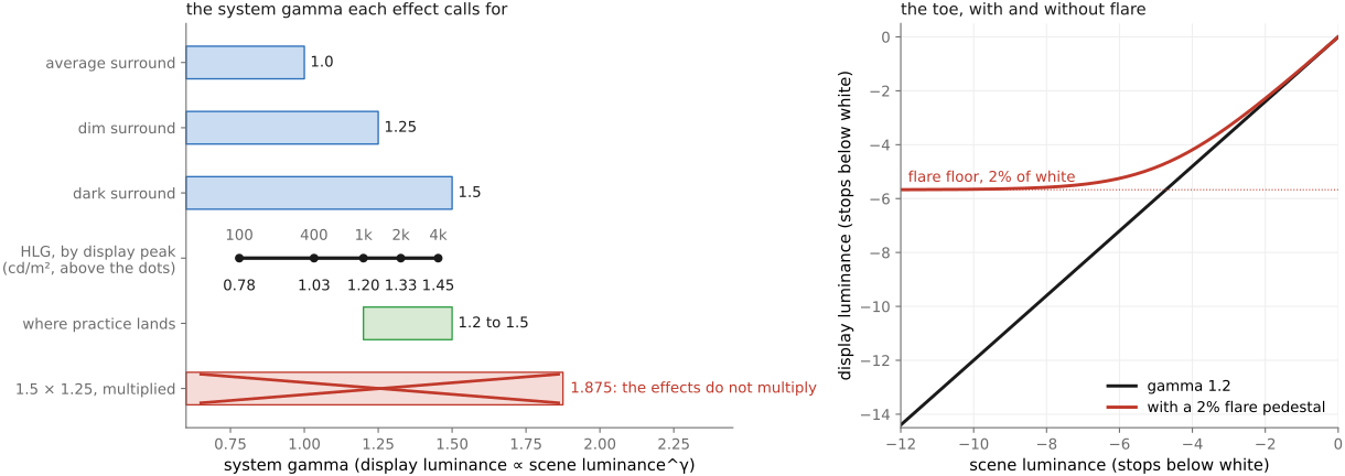
These effects are not independent and must not be multiplied together. Bartleson and Breneman's surround figures were measured at particular luminance levels, so their 1.25 and 1.5 already contain part of the Stevens effect; multiplying 1.5 by 1.25 gives 1.875, far above anything used in practice. Surround and absolute level are partly the same adaptation probed two ways. In practice, surround and level together land in a band from about 1.2 to 1.5; flare shapes the toe rather than contributing a global factor; and the Hunt effect acts on a different axis entirely, chroma rather than luminance.
What remains genuinely aesthetic is narrower than it appears: where middle gray is anchored, how the compression is split between shadow crush and highlight roll-off, and how soft the knee is. The last is the actual filmic look, and it has no perceptual justification. It came from emulsion chemistry, grain statistics at low exposure and dye saturation at high exposure, and was then selected because people liked it (Chapter 18.9, High dynamic range in traditional photography, Chapter 18.8, Display rendering transforms and color).
Figure 18.1.2 collects the values.
18.1.3 What local tone mapping relies on⧉
The local methods of the following chapters rest on three properties of spatial vision.
The visual system responds to local contrast far more than to absolute level. Center-surround receptive fields compare a region with its neighborhood, and contrast sensitivity is band-pass: we detect a grating of moderate spatial frequency at much lower contrast than a very slow variation across the visual field (Chapter 3.4, Spatial and temporal vision). A slow gradient of illumination across a room is barely noticed, while a small edge is seen clearly.
Lightness constancy discounts illumination. We judge the reflectance of a surface by comparing it with its surroundings, so a white page in shadow still looks white (Chapter 3.3, Adaptation and constancy). Illumination tends to vary slowly or change abruptly at shadow boundaries, while reflectance carries the texture. Compressing the large-scale variations of a radiance map, mostly illumination, while keeping its local contrast, mostly reflectance, therefore changes what the viewer perceives about the lighting much more than about the surfaces. That is the rationale behind every base/detail method.
The eye adapts locally and moves. Each fixation adapts to a region of the scene a degree or two across, and a viewer scanning a high-contrast scene sees each part at a different adaptation. A local operator is a crude imitation of that process frozen into one image, and the size of the neighborhood it uses plays the role of the adaptation field Pattanaik et al. 1998.
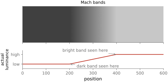
The same properties explain the failures. Edges are where the visual system concentrates its attention: Mach bands (Figure 3.4.1) and the Cornsweet illusion show that it reads contrast at an edge and fills in the regions on either side. A halo, a band of false brightness along a strong edge, is therefore conspicuous, which is why fifteen years of research went into decompositions that respect edges. And because we judge large regions relative to one another, pushing local contrast too far flattens the global relationships, a dark sky ending up as bright as a lit facade, which produces the overprocessed "HDR look".