16.8 Video, bursts, and lucky imaging🔗⧉

A long exposure of a planet averages changing atmospheric distortion as well as collecting photons. Short frames preserve some of that variation: a subset can have sharper detail than the full average. Those frames still contain shot and read noise, and their usefulness depends on exposure, target brightness and seeing.

Lucky imaging scores short exposures, selects useful frames, registers them and combines them (Law et al. 2006). Selection favors sharper atmospheric states; stacking reduces noise among the survivors. The retained fraction is a parameter to evaluate, not a universal few percent.

16.8.1 Atmospheric seeing: why one long exposure fails🔗⧉

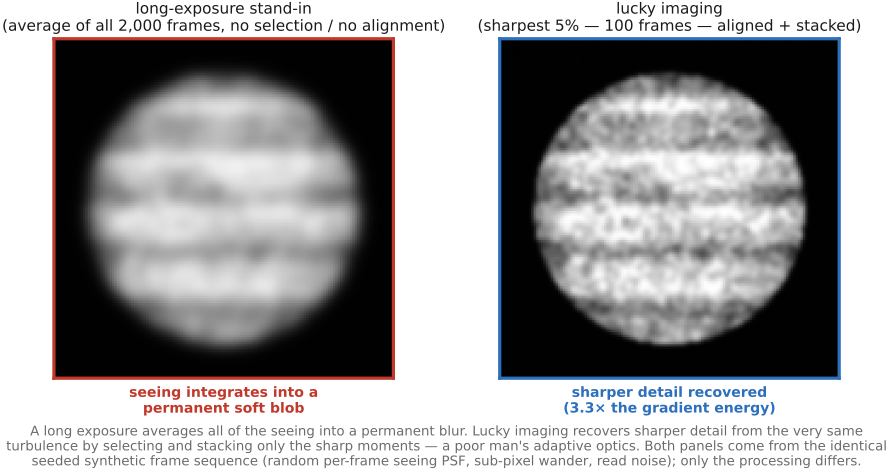
Point a telescope at a planet and you are looking up through kilometers of turbulent air. The atmosphere is not a uniform sheet of glass; it is a churning stack of cells at slightly different temperatures, and therefore slightly different refractive indices. A star's wavefront, flat by the time it reaches the top of the atmosphere, gets scrambled on the way down: different patches of the wavefront are delayed by different amounts, so the image they form wanders and smears as the cells drift and boil. This is the seeing, and it changes on a timescale of milliseconds. The consequence for a long exposure is fatal: the shutter is open for the duration of thousands of these atmospheric states, so the recorded image is the time-average of thousands of differently-distorted instantaneous images. Mathematically, a single long exposure is the true scene convolved by the time-averaged seeing point-spread function (PSF),

and $\overline{\text{PSF}}$ is a soft, broad blob, with width set by the atmosphere, not the telescope. Without wavefront correction, long-exposure resolution can be seeing-limited even with a large telescope (Figure 16.8.2⛶ fullscreen).

Short exposure freezes a turbulence state, but that instantaneous PSF can still be broad or speckled. Fried's coherence length $r_0$ characterizes the wavefront variation (Fried 1978). The chance of a nearly diffraction-limited exposure depends strongly on telescope diameter relative to $r_0$, wavelength and exposure duration. Selection is most useful when sufficiently good frames occur and can be identified.

16.8.2 Shoot thousands, keep the sharpest🔗⧉

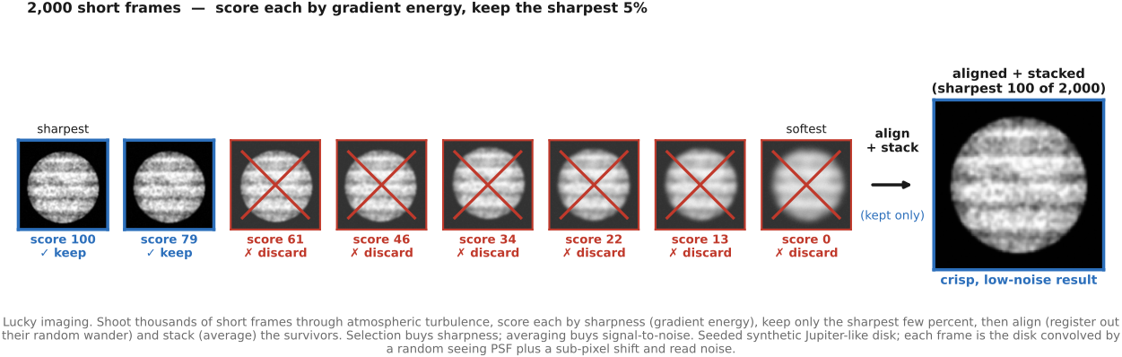
So flip the capture strategy. Instead of one long integration, record a high-frame-rate video, meaning thousands of short exposures, each frozen against the seeing, and treat it as a stack to be curated. The exposures are short enough that any single frame caught the atmosphere in essentially one state: some frames are badly distorted, most are mediocre, and a few are crisp. The task is to find the crisp ones, and that means putting a number on sharpness so the frames can be ranked.

The sharpness score is exactly the measure built for focal stacks: a region is sharp when it carries local high-frequency energy, and defocus or seeing-blur is a low-pass operation that destroys it. So score each frame by its gradient energy (or high-frequency power, or local contrast),

a single number per frame that is large for crisp frames and small for smeared ones. Then rank all the frames by $s_i$ and keep only the top $k\%$, with the retained fraction chosen for the sequence:

Raw gradient energy also increases with noise and sharpening. Use a common region, stable intensity normalization and a score tested against those effects. For small targets, local or reference-star quality measures can be more reliable than whole-frame energy. A high score alone does not establish a sharp atmospheric PSF.

Everything else is discarded. This is pure frame selection: "decide later" applied to the time axis, with the decision being which moments of atmosphere to trust (Figure 16.8.1⛶ fullscreen).

This is a form of Chapter 28.3, Auto curation with a narrowly defined target: select frames that improve the reconstructed image. Bright compact targets make fast acquisition and scoring easier. Stellar lucky imaging and combinations with adaptive optics extend the method beyond amateur planetary work; the signal available for scoring matters as much as the final object's brightness. Amateur planetary imagers run the whole pipeline with free tools: a video of a few thousand short frames is captured with a small astronomy camera, AutoStakkert! scores, aligns and stacks the best of them over many local patches, and RegiStax sharpens the stack with wavelet-band gains, the multiscale detail boost of Chapter 6.6, Pyramids and wavelets.

16.8.3 Align and stack the survivors🔗⧉

Register the selected frames before combining them. Their PSFs can still differ, and atmospheric motion can require local rather than global alignment. Define $\mathbf d_i$ as the shift applied to source frame $i$ to align it with the reference: the registered image samples $I_i(\mathbf x-\mathbf d_i)$ (Chapter 12.1, Brute force).

With the keepers aligned, the combine is the plainest tool in the part, the average from Chapter 13.2, Denoising by averaging:

The independent-noise averaging law is a reference case. Selection uses the observed data and surviving PSFs still differ; interpolation and calibration introduce further dependencies. A selected stack uses fewer photons than the complete acquisition and can incur more read noise than one long exposure. Compare sharpness and noise at fixed total capture time.

Sweep the retained fraction and inspect the final result rather than treating every survivor as perfectly sharp. Local registration can reduce atmospheric distortion within patches; it does not correct every wavefront error. Record any post-stack sharpening separately from the selection and averaging.

Sharpness selection and registration solve different problems. Imagine two selected frames whose fine planetary markings are individually clear but displaced by half a pixel. Averaging them at their original coordinates softens those markings, spending the sharpness gained by selection. Registering them first lets the scene contributions coincide while independent noise varies. Atmospheric distortions can differ across the field, so matching one feature globally may leave another misaligned. Local registration addresses that spatial variation, but must avoid fitting noise or changing real structure. Selection, alignment, and averaging each need to be checked separately.

16.8.4 A poor man's adaptive optics🔗⧉

Adaptive optics measures and compensates wavefront distortion during capture. Lucky imaging selects favorable recorded states. They spend different resources and can be combined; selection is not a universal substitute for wavefront correction (Law et al. 2006).

Short-exposure SNR, camera readout, seeing statistics and field size limit the gain. Different field regions can be sharp at different instants, motivating local alignment or selection. A faint extended object may supply insufficient detail for frame scoring even when a nearby reference star supports it.

When every frame is blurred, selecting a few need not use the data well. Model a registered static burst as $y_i=A_i x+n_i$ with a different known blur $A_i$ per frame. Under independent Gaussian noise, combine the constraints through

For periodic convolutions with responses $H_i$, the data constrains each frequency through $\sum_i|H_i|^2/\sigma_i^2$. A zero in one frame can be supplied by another; a common zero remains unobserved. This is different from aligning frames and averaging them as if they had identical sharpness.

Aittala and Durand learn to fuse differently blurred bursts with a permutation-invariant network (Aittala & Durand 2018 (permutation-invariant burst deblurring); Chapter 14.3, Learned burst methods). Order invariance does not by itself solve registration or identify a sharp target time in a moving scene. For video output, add temporal confidence, history reset and playback evaluation (Chapter 13.10, Video denoising).

A long exposure combines many instantaneous atmospheric distortions into one blurred image. Short exposures retain their variation: some frames are sharper, and some regions may be sharper in different frames. Rank or weight those observations, align them, and combine the useful evidence. The method can then spend less weight on strongly distorted measurements rather than committing to their average during capture.

Discarding frames also discards photons. Selecting one percent of a burst is costly when each exposure is noisy, and the sharpness statistic itself can be fooled by noise. The best retained fraction depends on brightness and seeing. Different lines of sight can experience different distortions, so one global frame score may be insufficient over a wide field. These are consequences of selection and spatial variation, rather than a categorical prohibition on every faint target.

A deformable mirror changes the wavefront before photons are recorded; frame selection chooses among states already recorded. The first requires sensing and controlling the distortion in time to correct it. The second can defer its decision until the full sequence is available, but spends photons on rejected frames and succeeds only when useful states occur. This is a concrete example of exchanging optical control for capture diversity and computation, rather than two algorithms applied to the same fixed measurement.