16.6 Defocus, and undoing what the lens softened⧉
A foreground portrait and its distant background can have different defocus responses. A single deconvolution may improve one depth while introducing errors at another. Motion blur can also vary spatially; the distinction here is that defocus depends on aperture and scene depth.
Defocus carries depth information under a calibrated optical model, but depth and texture can be ambiguous in one image. Additional focus settings or dual-pixel views provide further constraints rather than an exact operator for free.
16.6.1 The defocus PSF, and why one deconvolution is wrong⧉
For a point at distance $z$ and a lens focused at $z_f$, geometric optics gives a circle of confusion whose diameter grows with the aperture and with how far $z$ is from $z_f$. The PSF is roughly that disc, softened by diffraction and shaped by the aperture's actual outline, which is why bokeh takes the shape of the blades.
Under a thin-lens model with focal length $f$, entrance-pupil diameter $D$, focus distance $z_f>f$ and object distance $z>f$, the sensor-plane circle diameter is
Divide by pixel pitch for a diameter in pixels. The dependence is on reciprocal depth, not simply distance from the focus plane. A geometric disc is an approximation; diffraction and aberrations alter its response.
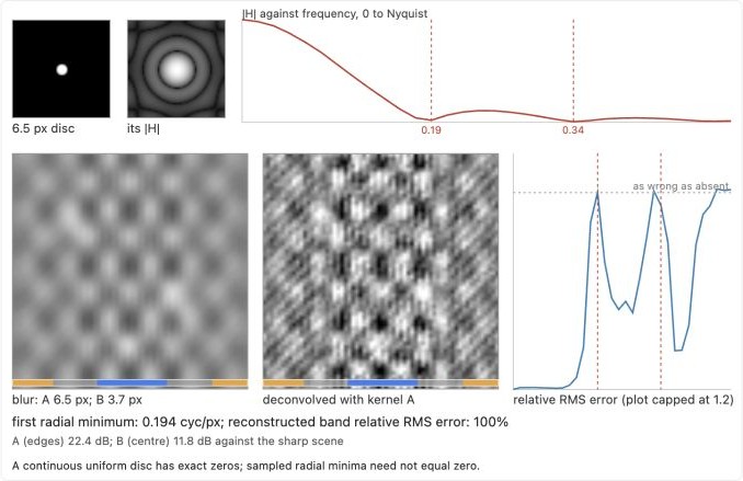
The disc has a property that matters more than its shape: its transfer function has zeros. A uniform disc's Fourier transform crosses zero at a set of radii, and at those frequencies the measurement contains nothing at all, not a small amount. No prior recovers a frequency that was multiplied by zero, which is the sharpest statement in this part of the difference between attenuated and annihilated (Chapter 16.1, What blur is, and what deblurring can undo). Uniform linear motion also has sinc zeros. The location and strength of the responses, together with noise, determine recoverability in either case.
A single convolution can be appropriate for one depth plane with sufficiently uniform optics. Across depths or occluding boundaries, a more complete model is needed; null components remain unconstrained by that one observation.
16.6.2 Estimating the blur field⧉
A depth map helps specify blur only with aperture, focus, lens response and visibility. At depth boundaries, foreground occlusion changes which rays reach the sensor, so independent local disc blurs are incomplete. Several measurements can constrain the field:
From the single image. Estimate a defocus map by measuring local sharpness, or by how much a local edge is spread, and convert it to a blur radius. It is the same estimation problem as blind deblurring restricted to a one-parameter family, which makes it far better posed, and it fails in the same places: flat regions, where there is nothing to measure the blur on, and depth discontinuities, where two blurs overlap.
From two images. Different focus or aperture settings can constrain defocus through their relative image formation. The scene must align and remain sufficiently stable; exposure changes and spectral zeros complicate a direct ratio. The result remains an estimate under a model.
From dual-pixel data. Two sub-aperture views provide a small-baseline disparity cue related to defocus (Abuolaim & Brown 2020). Calibration, texture, aperture and noise determine how informative it is. Flat regions and occlusions remain difficult, and the views are not generally identical images related only by a shift. A learned model can use both without explicitly recovering a perfect depth map.
The sign of a dual-pixel disparity can help distinguish which side of the focus plane a point lies on. A symmetric defocus disc alone does not provide that sign: comparable blur sizes can arise in front of and behind the chosen focus. Splitting the aperture changes the measurement so that the two subviews can resolve part of that ambiguity. Their usefulness still depends on texture and the calibrated lens response.
16.6.3 Lens softening, which is a different problem with the same shape⧉
Even in focus, a lens is not perfect. Aberrations spread a point into a small PSF that varies across the field, differs between sagittal and tangential directions, changes with aperture and focus distance, and differs per wavelength (Chapter 22.3, Measuring lens quality).
PSFs can be calibrated across field position, wavelength, aperture and focus. Lens copies, stabilization state and capture conditions can change them. A lens profile is not automatically a measured spatial deconvolution kernel; distortion and shading profiles serve different purposes.
The limits are the same as everywhere else in this part. The correction is only as good as the calibration, which assumes this copy of the lens matches the profiled one. It amplifies noise in proportion to how much it sharpens, which is Chapter 16.2, Non-blind deconvolution's tradeoff with a smaller kernel. And it cannot restore what the lens did not transmit, so past the diffraction limit it is inventing.
16.6.4 Engineering the blur instead of fighting it⧉
A patterned aperture can improve the transfer response over selected frequencies and provide depth-dependent signatures. Wavefront coding can make the PSF less sensitive to defocus over a designed range. Finite aperture still imposes an optical cutoff, and neither approach guarantees a zero-free response at every frequency or an unambiguous depth estimate.
Both are developed where they belong, in Chapter 33.3, Coded aperture and Chapter 33.1, Wavefront coding. They are mentioned here because they are the answer to this chapter's problem rather than an unrelated topic: if the operator is bad, and you own the optics, fix the operator.