16.4 Blind deblurring⧉
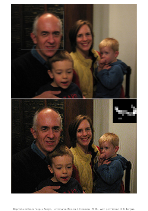
A streetlamp smeared into a short curve suggests the exposure motion, but a real lamp has extent and may saturate. Inferring the point-spread function from the photograph is therefore an estimation problem. We begin with one spatially invariant kernel; Chapter 16.5, Spatially varying blur relaxes that approximation.
16.4.1 Estimating the kernel and the image at once⧉
With an unknown kernel, $Y=K*X+n$ is linear in $X$ for fixed $K$ and linear in $K$ for fixed $X$, but bilinear in the pair. The kernel usually has far fewer parameters than the image; adding it does not double the unknown count. Scale and translation ambiguities remain unless conventions or constraints fix them.
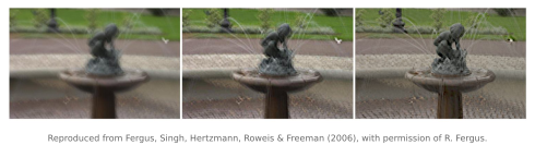
Knowing one variable makes the other subproblem simpler, not automatically easy. Kernel estimation from a known image still needs informative structure, adequate signal and constraints; division by that image's spectrum fails where it is weak. Known-kernel image recovery remains noise-sensitive (Figure 16.4.3).
16.4.2 Can you measure the kernel instead?⧉
A gyroscope supplies angular motion, while accelerometers and calibration can contribute additional information (Joshi et al. 2010). Exposure synchronization, sensor-to-camera calibration, stabilization motion, bias, rolling shutter and scene depth determine the accuracy of the resulting blur estimate. Use inertial data as a constraint or initialization when appropriate; a universal claim that it is always too coarse or always sufficient is unwarranted.
To turn angular-velocity samples into image blur, first express them in the camera's coordinate system and integrate over the actual exposure interval. Project a scene direction through the resulting orientations to obtain its image trajectory, then accumulate the time spent along that trajectory into a blur model. An exposure timing offset changes which part of the recorded motion is used. Image stabilization can make lens or sensor motion differ from the body motion measured by the IMU. These are concrete calibration problems, not reasons to dismiss inertial measurements: synchronized and calibrated measurements can constrain an image-based estimate substantially.
16.4.3 Why the obvious optimizer fails⧉
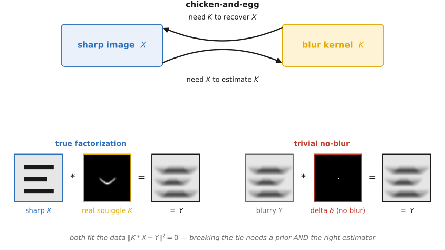
Even in the noiseless model, factorization is ambiguous. Both $Y=X*K$ and $Y=Y*\delta$ fit exactly, where $\delta$ is the identity kernel. With noise, the latter still fits the recorded data exactly while the true latent image and kernel generally leave a residual. A data term alone therefore cannot distinguish a sharp latent image from the observation explained by an identity kernel.
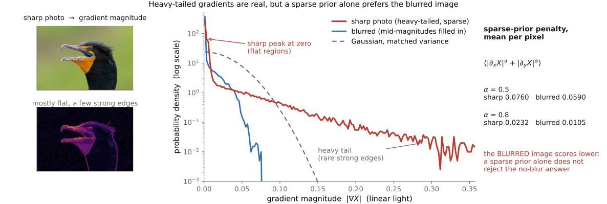
Image and kernel priors can distinguish explanations, but a sparse-gradient image prior alone does not necessarily prefer the true sharp image in joint MAP. Blurring changes gradient magnitude and count together; the prior's total cost can favor the no-blur explanation. This tension is central to Levin et al.'s analysis (Levin et al. 2009), and the histogram alone does not resolve it.
The objective puts data-fit and two priors together:
Here $\rho$ can sum $|g|^\alpha$ over gradients and $\psi$ represents kernel regularization. Enforce nonnegativity, unit sum and a finite support when those match the PSF model. A physical motion PSF is an exposure-weighted occupancy of projected positions, not necessarily a thin connected curve after finite sampling or other blur. The joint problem remains nonconvex.
16.4.4 Two ways to solve it⧉
Two approaches, with an important caveat between them:
- Alternating minimization. The obvious approach. Fix $X$, solve for $K$; fix $K$, do a non-blind deconvolution for $X$; repeat. In practice this is run coarse-to-fine: estimate the kernel on a heavily downsampled image first, where the blur is small and the problem is easy, then refine up the pyramid to full resolution:
K ← δ                                  # start from "no blur"
for each pyramid level, coarse to fine:
    initialize X from this level of Y on the first level
    otherwise resize X and K, scale kernel support, and renormalize K
    repeat until converged:
        X ← argmin_X ‖K * X − Y‖² + λ·ρ(∇X)     # non-blind deconv, K fixed
        K ← argmin_K ‖K * X − Y‖² + μ·ψ(K)      # fit kernel, X fixed
return non-blind deconvolution of Y with the final K
It is simple and often works, but it can collapse to the trivial delta-kernel solution if the prior is not handled carefully: the optimizer slides toward "no blur" exactly as warned above.
Marginal kernel estimation instead integrates over image uncertainty. It scores a kernel by the total evidence of possible images rather than the density of one selected pair. This can avoid the no-blur bias of particular joint-MAP formulations, but depends on the prior, likelihood and approximation:
The integral is generally expensive; variational inference is one approximation. A lower-dimensional kernel can be better constrained than all image pixels jointly without becoming identifiable for every scene. Flat images, severe noise and model mismatch remain ambiguous.
The attribution is straightforward. Fergus, Singh, Hertzmann, Roweis & Freeman (2006) Fergus et al. 2006, "Removing Camera Shake from a Single Photograph," established blind deblurring on real photographs, using a natural-image gradient prior together with variational inference to estimate the kernel. Levin, Fergus, Durand & Freeman (2007) Levin et al. 2007 clarified the role of the sparse prior in non-blind deconvolution, and Levin, Weiss, Durand & Freeman (2009) Levin et al. 2009 gave the canonical evaluation: the careful analysis of why naive joint MAP fails and why marginalizing over the image is what actually works. In a blind problem, the estimator design, not just the prior, is load-bearing. Chapter 16.7, Learned deblurring includes models that predict the image directly as well as methods retaining explicit operators. They do not all follow this marginal-kernel structure L7.6.
The distinction is between a high peak and substantial probability mass. Joint MAP selects one image/kernel pair at a peak of their posterior density. Marginal estimation asks how much image probability supports a kernel after integrating across alternatives. A kernel supported by a broad range of plausible images can therefore outrank one whose best-fitting image alone has a higher density. This is why changing the estimator can change the chosen kernel even while keeping the likelihood and prior fixed.