16.1 What blur is, and what deblurring can undo⧉
Motion during an exposure spreads the image of a point along a trajectory. Defocus and diffraction also spread points, and atmospheric turbulence can change the response during capture. These mechanisms affect both resolution and the model needed for reconstruction.
A convolution $Y=K*X+n$ describes spatially invariant blur. It can be a useful local approximation for motion, defocus or atmospheric blur; depth changes, rotation and occlusion often require a spatially varying operator. The desired $X$ must be defined, for example as the sharp image at a reference exposure time.
This chapter is about what that convolution did to the information, because that decides what any later chapter is entitled to claim. Some frequencies were attenuated and can be brought back at a price paid in noise. Some were multiplied by zero and are gone, and no prior, no network and no amount of regularization returns them. Knowing which is which, for a given blur, is the difference between deblurring and inventing.
16.1.1 Why naive inversion fails⧉
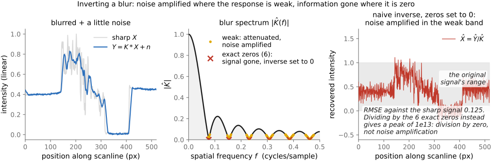
Start with the easy version to see exactly where it breaks. The blur is a known kernel $K$, there is no noise, and the observed image is $Y = K * X$. Convolution is a per-frequency multiply (this is L6.8: convolution diagonalizes in Fourier, from Part 6, Linear methods and Fourier analysis), so in the Fourier domain $\hat Y = \hat K \,\hat X$, and, where the response is nonzero under the chosen boundary model, recovering the sharp image is one division: $\hat X = \hat Y / \hat K$, then transform back. An exact zero leaves that component undetermined.
With noise, the inverted error at a frequency is its measured error divided by the blur response. A response of 0.01 multiplies the noise amplitude there by 100 and its power by 10,000. Blur responses can have directional zeros and lobes; they need not decrease monotonically with frequency. Figure 16.1.1 illustrates an ill-conditioned example.
For a general matrix $A$, small singular values identify weakly observed combinations of image samples. For periodic convolution, Fourier modes provide the corresponding frequency picture. For a spatially varying operator, these combinations are not simply low- and high-frequency bands.
Regularization limits amplification of weakly measured components (L7.8). Its result can be biased, and a prior-selected value in a null space is not an extra measurement.
The same calculation applies beyond convolution. Write a forward matrix as $A=U\Sigma V^{\mathsf T}$. Projecting the observation onto the left singular vector $u_j$ gives $u_j^{\mathsf T} Y=\sigma_j v_j^{\mathsf T} X+u_j^{\mathsf T} n$. Direct inversion divides this scalar by $\sigma_j$. A small singular value therefore amplifies the projected noise; a zero singular value leaves the corresponding image component unmeasured. For shift-invariant blur, the Fourier representation provides the analogous componentwise calculation. For spatially varying blur, the singular-vector argument still explains the instability even though a single Fourier division no longer solves the problem.
16.1.2 The fix, stated once⧉
Balance the data fit against an image model rather than inverting every response equally. Wiener filtering Wiener 1949 gives the minimum expected squared-error linear estimate for specified second-order statistics. More expressive priors can treat edges and texture differently (Chapter 16.2, Non-blind deconvolution, Chapter 16.3, Priors for deconvolution).
16.1.3 Which space to deblur in⧉
The physical blur model is linear in radiance or expected photoelectron signal before clipping. Use that domain for a physical deconvolution. Decoding a known display transfer function does not undo an unknown local tone map or earlier sharpening. A network trained directly on encoded images can model that processing empirically, but its input is not the same linear convolution problem.