15.10 Quad-Bayer and Nona-Bayer processing⧉
Most phone sensors with small photosites group them: Quad-Bayer puts four photosites under each color filter, in $2 \times 2$ blocks, Nona-Bayer nine, in $3 \times 3$ blocks, and the largest sensors use $4 \times 4$ blocks, the general Q×Q pattern (Chapter 15.5, Alternative color filter arrays). In low light the sensor bins each block into one pixel and hands the pipeline an ordinary Bayer mosaic, and everything in the earlier chapters of this part applies. This chapter is about the other mode, full resolution, where every photosite is read and something has to turn the grouped mosaic into a color image.
Two routes exist. The one phones mostly use is to remosaic, estimating a conventional Bayer mosaic from the grouped one so that the camera's Bayer image signal processor can take it from there. The other is to demosaic the grouped layout directly. Every published direct method we know of is learned, and the comparisons that exist favor it. The reasons, and why the industry took the detour anyway, are what this chapter is about.
15.10.1 Why the classical methods do not transfer⧉
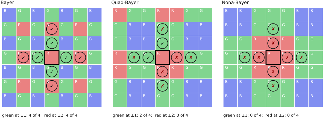
The edge-directed machinery of Chapter 15.1, Basic traditional demosaicking is built on the geometry of the Bayer lattice. At a red site, green is measured immediately to the left and right and immediately above and below, and red again two pixels away in each direction. Hamilton–Adams uses exactly those samples: the green difference across the site, corrected by the second difference of red at distance two, once horizontally and once vertically, and picks the direction with the smaller variation.
A Quad-Bayer mosaic has none of that. Its tile is four pixels wide, with rows RRGG, RRGG, GGBB, GGBB. At the top-left red of a block, the pixel on its right is red and the one on its left is green; the next green on the right is two pixels away; and two pixels away on either side there is green, not red. The symmetric pair of green neighbors and the same-color samples at distance two, which every step of Hamilton–Adams reads, do not exist. Green arrives in $2 \times 2$ clumps on a lattice twice as coarse, and a gradient measured across a clump boundary mixes a change of color with a change of scene. Nona-Bayer is worse: the center of a $3 \times 3$ block is a full pixel from the nearest other color in every direction (Figure 15.10.1).
There is no natural analog of the Bayer rules on this lattice, and we know of no published classical demosaicker that works on the grouped layout directly; recent papers state that conventional demosaicking algorithms cannot operate on these patterns Tedla et al. 2025 (unified joint demosaicking and denoising, Single/Quad/Nona). The industry went around the problem instead.
15.10.2 Remosaicking: making the sensor look like Bayer⧉
A phone's image signal processor is hardware, and its demosaicker, denoiser, sharpening and every tuning table downstream were built and calibrated for Bayer input. A new sensor layout that required a new processor would be expensive, so the sensor is made to look like the old one. Remosaicking estimates, at every photosite, the value a Bayer sensor would have measured there, and hands that estimate to the unchanged pipeline. It often runs on the sensor chip itself: Sony's first 48-megapixel Quad-Bayer sensor, for instance, converted its array to Bayer with its own on-chip signal processing.
Remosaicking is interpolation. At some sites the Quad color and the Bayer color agree and the measurement passes through; at the others the remosaicker has to estimate a color that was not measured there. For Quad-Bayer that is 10 of the 16 sites in each tile, 62.5% of the image, and for Nona-Bayer half of it (Figure 15.10.2). The published remosaicking algorithms are proprietary, but the idea can be sketched with the tools of Chapter 15.1, Basic traditional demosaicking: at a site that needs a color it did not measure, choose a direction from the local gradients, then interpolate that color along it, corrected by a color difference estimated in the same direction.
remosaic(quad):                                   # a minimal sketch, not a vendor's algorithm
  Y = rough_luma(quad)                            # e.g. a small box filter over the mosaic
  for each site p:
    want = bayer_color(p);  have = quad_color(p)
    if want == have:
      out[p] = quad[p]                            # measured: pass it through
      continue
    # choose a direction on the rough luma, since same-color neighbors
    # sit at distance 1 inside a block but 2 or more across blocks
    dir = H if variation(Y, p, H) < variation(Y, p, V) else V
    if want does not occur on the line through p along dir:
      dir = the other axis                        # a Quad row carries only two colors
    if want occurs on neither line:
      out[p] = quad[p] + window_difference(quad, p, want, have)   # small window fallback
      continue
    # form the difference where WANT was measured: its sample minus HAVE
    # interpolated along the same line there; then interpolate that
    # difference to p along dir and add it to what p measured
    D = [quad[q] - interp_along(quad, q, have, dir) for q in sites_of(want, line(p, dir))]
    out[p] = quad[p] + interp_along_from(D, p, dir)
  return out                                      # a Bayer mosaic, 62.5% estimated
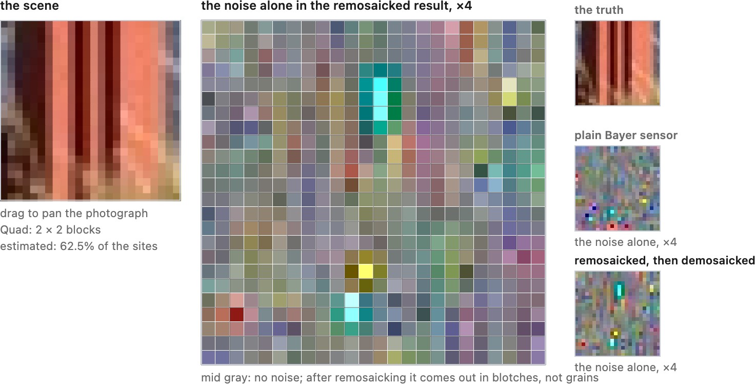
The result is a mosaic in which most values are estimates that look like measurements. The Bayer demosaicker downstream cannot know which is which, so it interpolates between estimates as though they were data, and an error the remosaicker made, a wrong direction on a fine texture for instance, is copied into the missing colors of the neighbors. Noise is transformed too: the remosaicker mixes neighboring samples, so the noise it hands on is correlated and no longer matches the model the Bayer denoiser was tuned for.
This is why learned remosaickers fold denoising in. The MIPI 2022 challenge posed the task exactly as a phone needs it, a noisy Quad-Bayer mosaic in and a clean Bayer RGGB mosaic out MIPI 2022 (quad-Bayer remosaic challenge) ⚠️, and Zeng and colleagues' network does both jointly, a remosaicking branch and a denoising branch producing a Bayer mosaic that a conventional pipeline can consume Zeng et al. 2024 (joint Quad-Bayer remosaicking and denoising).
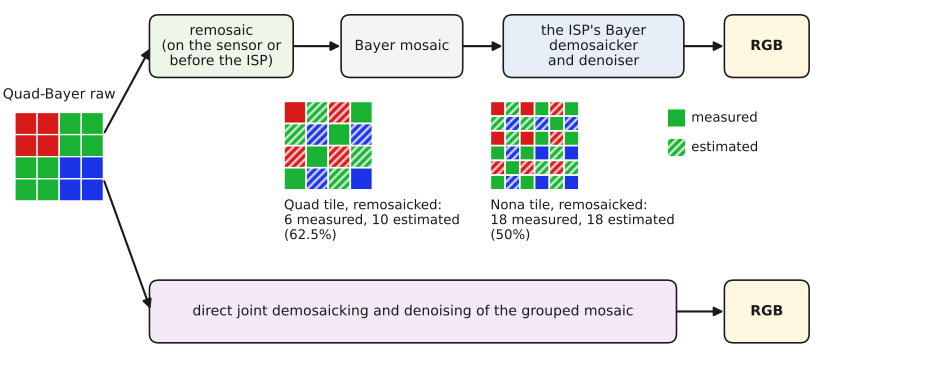
Figure 15.10.3 runs the sketch step by step. The difference has to be formed where the wanted color was measured, not by interpolating the two colors separately, which takes them from different places: on a slow gray gradient that version is already off by about a tenth of the range. For Quad-Bayer the fallback window is needed at 72 of every 576 sites, for Nona-Bayer at 32. On a photograph of a bridge, the remosaicked and demosaicked result scores 17.8 dB, against 26.9 dB for a plain Bayer sensor of the same pixel count demosaicked the same way, and its color noise is stronger and correlated two pixels away (0.28, against 0.03 on Bayer), the correlation the Bayer denoiser downstream is not built for.
15.10.3 Demosaicking the grouped layout directly⧉
The direct route maps the grouped mosaic to a full color image in one step, and every method that takes it is a network. The first we know of came from Samsung. Kim and colleagues' duplex pyramid network demosaics Quad-Bayer without a remosaicking stage, with a very large receptive field aimed at the large-scale artifacts that grouped layouts produce, color moiré at the lower frequencies of Chapter 15.3, Mosaics and aliasing, while staying cheap enough for a phone Kim et al. 2019 (duplex pyramid network, Quad-Bayer). A follow-up applied the same structure to Samsung's 108-megapixel Nona-Bayer sensor Kim et al. 2021 (Nonacell demosaicking).
Most later work folds denoising in, for the reason Chapter 15.8, Joint demosaicking and denoising gives: a grouped sensor is used at full resolution in good light, but its photosites are small and noisy. Sharif, Naqvi and Biswas map the noisy Quad-Bayer mosaic directly to a clean color image Sharif, Naqvi & Biswas 2021 (BJDD), the method most comparisons use as the Quad-Bayer baseline, and their SAGAN does the same for Nona-Bayer Sharif, Naqvi & Biswas 2021 (SAGAN, Nona-Bayer). PyNET-QxQ adapts a phone-scale network to general Q×Q patterns Cho et al. 2023 (PyNET-QxQ). Zheng and colleagues' DRNet gives one of its two encoders a first layer designed for the Quad arrangement Zheng et al. 2024 (DRNet, Quad-Bayer).
Two papers handle every layout with one model. Lee and colleagues' KLAP demosaics Bayer, Quad, Nona and Q×Q with a single network in which only about 1% of the filters are specific to the array, and its variant KLAP-M adapts at test time to artifacts of a real sensor that synthetic training data does not contain Lee et al. 2023 (KLAP, unified Bayer and non-Bayer). Tedla and colleagues' unified joint demosaicking and denoising adds three channels to the input that say, at each pixel, which color was measured there; the same network then serves Single-, Quad- and Nona-Bayer, and randomly masking out pixels during training also teaches it to fill in dead ones. They captured 638 raw photographs of difficult scenes for training and testing Tedla et al. 2025 (unified joint demosaicking and denoising, Single/Quad/Nona).
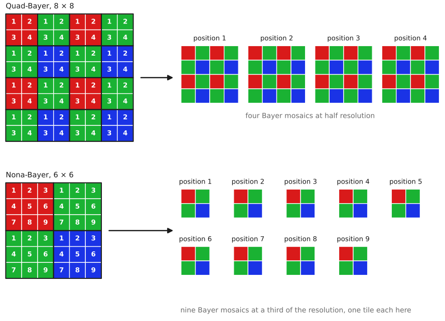
Much of the difficulty is in the representation, not in the problem. Take every second pixel of a Quad-Bayer mosaic, starting from the top-left pixel of each block: the result is an ordinary Bayer mosaic at half the resolution. There are four such sub-images, one for each position in the block, and all four are Bayer mosaics (Figure 15.10.4). Rearranging the input into those four planes, the pixel-unshuffle operation of many network libraries, gives a network built for Bayer the geometry it expects, and the same holds for Nona-Bayer with nine planes. The Bayer structure was in the data all along, sampled four times with small offsets; this is what makes a network designed for Bayer adaptable to grouped layouts with little more than a change at its input.
15.10.4 Remosaic or demosaic directly?⧉
The remosaicking route has a bottleneck built in. It must produce a mosaic with one value per pixel, so everything the grouped measurements say about a site has to be squeezed into the one color Bayer would have measured there, before the demosaicker sees any of it; and the estimates arrive without their uncertainty. Tedla and colleagues put the position directly: any remosaicking solution loses some information in converting a Quad- or Nona-Bayer mosaic into a Single-Bayer one. They then measure it. A hand-designed remosaicker followed by a Bayer demosaicking network falls far short of the same network trained to go directly from the grouped mosaic to color, and a learned remosaicker narrows the gap without closing it Tedla et al. 2025 (unified joint demosaicking and denoising, Single/Quad/Nona).
So the detour is a consequence of hardware, not a choice made for quality. It keeps a Bayer processor, and all the tuning invested in it, working with a new sensor. Where a phone runs a network on full-resolution stills anyway, as the introduction to this part describes, the direct route costs little extra and removes the intermediate mosaic. The same question arises for the rest of the pipeline in Chapter 15.9, Joint methods and the end-to-end pipeline: an intermediate representation that suits existing hardware is not necessarily the one that suits the reconstruction.
The MIPI challenges show the two framings side by side. Their 2022 Quad-Bayer track asked for remosaicking and denoising into a clean RGGB mosaic, the output a phone processor needs MIPI 2022 (quad-Bayer remosaic challenge) ⚠️. Their 2024 track used a hybrid event-vision sensor, a Quad-Bayer array with event-detecting pixels in place of some color ones, and asked for the color image directly, filling in the event pixels along the way; the winner, DemosaicFormer, goes coarse to fine, a demosaicking network followed by one that corrects the pixels the first got wrong Xu et al. 2024 (DemosaicFormer), and a later method separates the two jobs, first filling in the event pixels within the Quad mosaic and then demosaicking it, with lighter state-space blocks Zhou et al. 2025 (TSANet). Once the sensor departed far enough from Bayer that no Bayer processor would take it, the challenge was posed directly.
15.10.5 Split exposures within a block⧉
The four photosites of a Quad block can also be given different exposure times or conversion gains, so that one capture contains a short and a long exposure of nearly the same place (Chapter 17.1, Dynamic range and multiple-exposure capture). Reconstruction then joins demosaicking with high-dynamic-range merging and, if the exposures differ in length, with deblurring: the long exposure is cleaner and blurrier, the short one sharper and noisier. Zhao and colleagues design a network for such a dual-exposure Quad-Bayer sensor and train it on pairs synthesized from ordinary Bayer data Zhao et al. 2024 (dual-exposure Quad-Bayer). Neither remosaicking nor a Bayer demosaicker has a natural place for two exposures in one block, which is one more case for the direct route.