15.9 Joint methods and the end-to-end pipeline⧉
Reconstruction and rendering stages interact: denoising changes what sharpening sees, and tone mapping changes the visibility of residual noise. Training a complete pipeline against its final output can account for such interactions (Chapter 15.8, Joint demosaicking and denoising).
One design maps a raw mosaic directly to a rendered image. Another keeps named stages and trains some or all of them together. End-to-end training describes the optimization boundary, not a requirement that every intermediate representation be hidden.
15.9.1 What end-to-end learning gains⧉
PyNET (Ignatov et al. 2020 (PyNET)) and DeepISP (Schwartz et al. 2018 (DeepISP)) demonstrate learned raw-to-rendered processing. Their comparisons support performance on the evaluated cameras, targets and metrics; they do not establish superiority over every conventional pipeline.
Optimizing the composition allows a stage to adapt to the input it actually receives and the processing that follows. Gains can also come from stronger individual estimators and training data. Ablations are needed to separate these explanations. A differentiable pipeline can retain explicit white-balance, color and tone operations while learning other stages.
Learning to See in the Dark (Chen et al. 2018) demonstrates direct reconstruction from short-exposure raw input using long-exposure references. Its result depends on the capture model and paired training; it is not proof that every conventional pipeline necessarily discarded the recoverable information.
For example, a denoiser tuned only against a clean reference may leave a residual that becomes conspicuous after shadow brightening. A sharpening stage may amplify that residual. Training or tuning the composition lets the denoiser account for those later operations. The example does not require every stage to be a network: a differentiable tone curve or fixed sharpener can still influence the loss used to train the reconstruction stage. This is the system-level counterpart of unrolling a solver in Chapter 13.7, Learned denoisers.
15.9.2 What it costs⧉
An unconstrained raw-to-sRGB network may offer no documented intermediate representation for editing. That limits a conventional exposure or white-balance control unless the model was designed to support it.
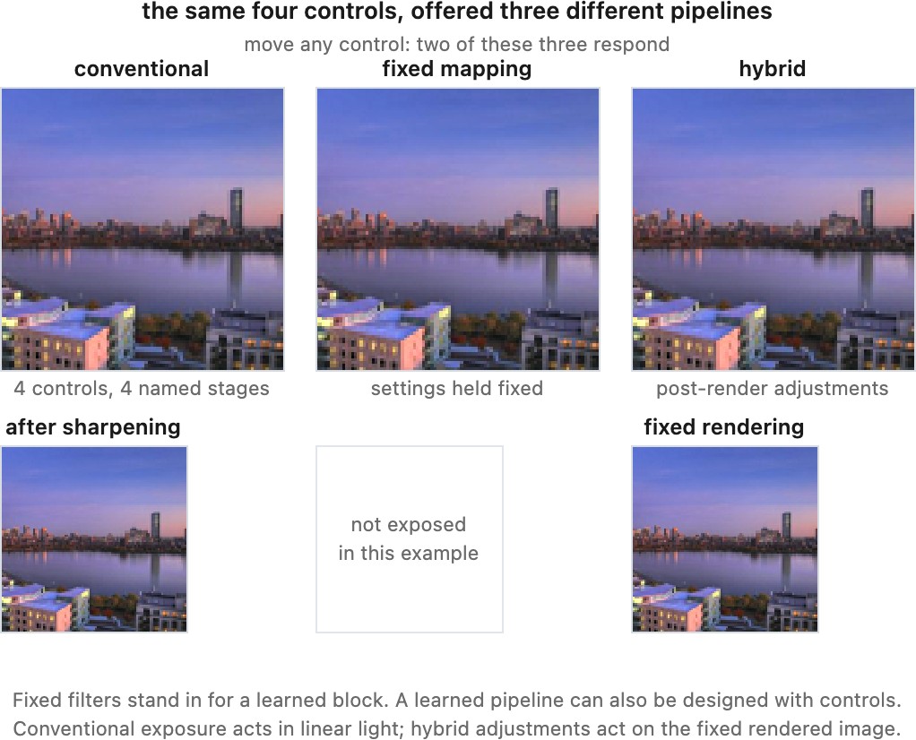
A photographer changes white balance after the fact, lifts shadows, sets a tone curve, and expects those controls to behave predictably and independently. Those controls exist because the conventional pipeline has named intermediate representations with meanings: linear light after demosaicking, white-balanced linear light after the gains, a colorimetric space after the matrix, a display encoding after the curve. Each control acts on one of them, and the type system of the color part is exactly what makes that reasoning possible.
A learned model can expose controls through conditioning inputs, explicit stages or a linear output representation. These controls need tests for predictable response, range and interactions. Retraining is not the only possible adjustment, but adding a slider after training does not guarantee meaningful control.
Other costs include debugging, regressions across subjects and cameras, runtime, memory and power. A model change can alter rendering beyond the cases that motivated it. Measure those effects at the target resolution and hardware.
15.9.3 Keeping a useful intermediate representation⧉
A practical architecture can learn early reconstruction while returning linear camera RGB, then use calibrated color conversion and explicit rendering controls. White balance or other gains may occur before, within or after reconstruction according to the model's convention.
Reconstruction has a physical target, but its regularization still trades detail against noise and can expose a useful strength control. Rendering adds choices about appearance. Separating the representations makes both kinds of control easier to interpret.
It also preserves the thing the book's color part spends four chapters building: an intermediate representation whose numbers mean something. A raw file remains editable because the pipeline after the raw stage is a set of documented operations on values with defined encodings, and that is what makes the same capture renderable two ways next year.
15.9.4 Where the field actually is⧉
For a deployable pipeline, specify the model's input units, CFA phase, supported cameras, output encoding and editable controls. Preserve raw data and record model versions so future rendering can start from the measurements. Published demonstrations and product descriptions provide examples, but do not reveal the complete pipeline of every camera or establish that no fully learned path has shipped.
15.9.5 Where demosaicking sits in the pipeline⧉
Demosaicking normally follows linearization, black-level correction, and defect handling. White balance and denoising may occur before it, after it, or jointly with it; a scalar CFA sample can already receive its channel's white-balance gain. A camera-to-output color matrix requires reconstructed channels. Nonlinear rendering and output encoding belong to the later appearance stages, as summarized in Chapter 8.12, Recap ISP, non-destructive editing.