15.2 Advanced traditional demosaicking🔗⧉

The methods below, published between the late 1980s and the mid-2000s, combine the two ideas of Chapter 15.1, Basic traditional demosaicking, edge direction and color differences, in different proportions, and hand-designed methods of this family are still what most cameras and phones run in their image signal processors, where a demosaicker must run on every preview and video frame, fast, small and predictable. Learned demosaicking has shipped mainly in desktop raw converters, such as Adobe's Enhance Details and DxO's DeepPRIME, which also denoises (Chapter 15.6, Learned demosaicking). Some phone pipelines avoid single-frame demosaicking altogether by merging a burst of raw frames directly onto a full-color grid (Chapter 14.2, Multi-frame super-resolution). Figure 15.2.1⛶ fullscreen runs ten of them side by side on the same mosaic, including the residual interpolation and ARI of this chapter, so each method's assumption can be seen where it fails.

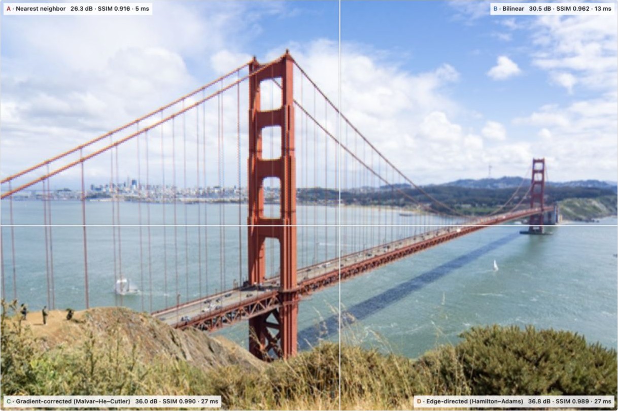
Nearest neighbor copies each missing value from a nearby sample of the right color, with no arithmetic. The name is loose, because most sites have several equally near samples of a given color: a red site has four green neighbors at the same distance, and four blue ones on the diagonals. An implementation breaks the tie with a fixed rule, usually by working tile by tile. In the lab's version, every pixel of a 2 × 2 tile takes that tile's one red and one blue, a green site keeps its own green, and the other two sites take the same one of the tile's greens. That makes it a close relative of the downsampling of Downsampling and bilinear interpolation, and how they fail: downsampling turns each tile into one pixel, and nearest neighbor is almost that same small image blown back up to full size by copying each value into the four pixels of its tile. The only differences are that the measured greens stay where they were and nothing is averaged. Nearest neighbor therefore keeps the pixel count but adds almost no detail over downsampling, and it keeps downsampling's flaw: each color is attributed to a place up to a pixel away from where it was measured, so every edge becomes a colored staircase, the strongest zipper of any method here. It costs nothing, which is why it survives in live previews and thumbnails. Bilinear interpolation (Downsampling and bilinear interpolation, and how they fail) averages instead of copying and fixes the misregistration in smooth regions, not at edges.

Figure 15.2.2⛶ fullscreen works through every method of this section on a small mosaic, one step per stage, starting with nearest neighbor.

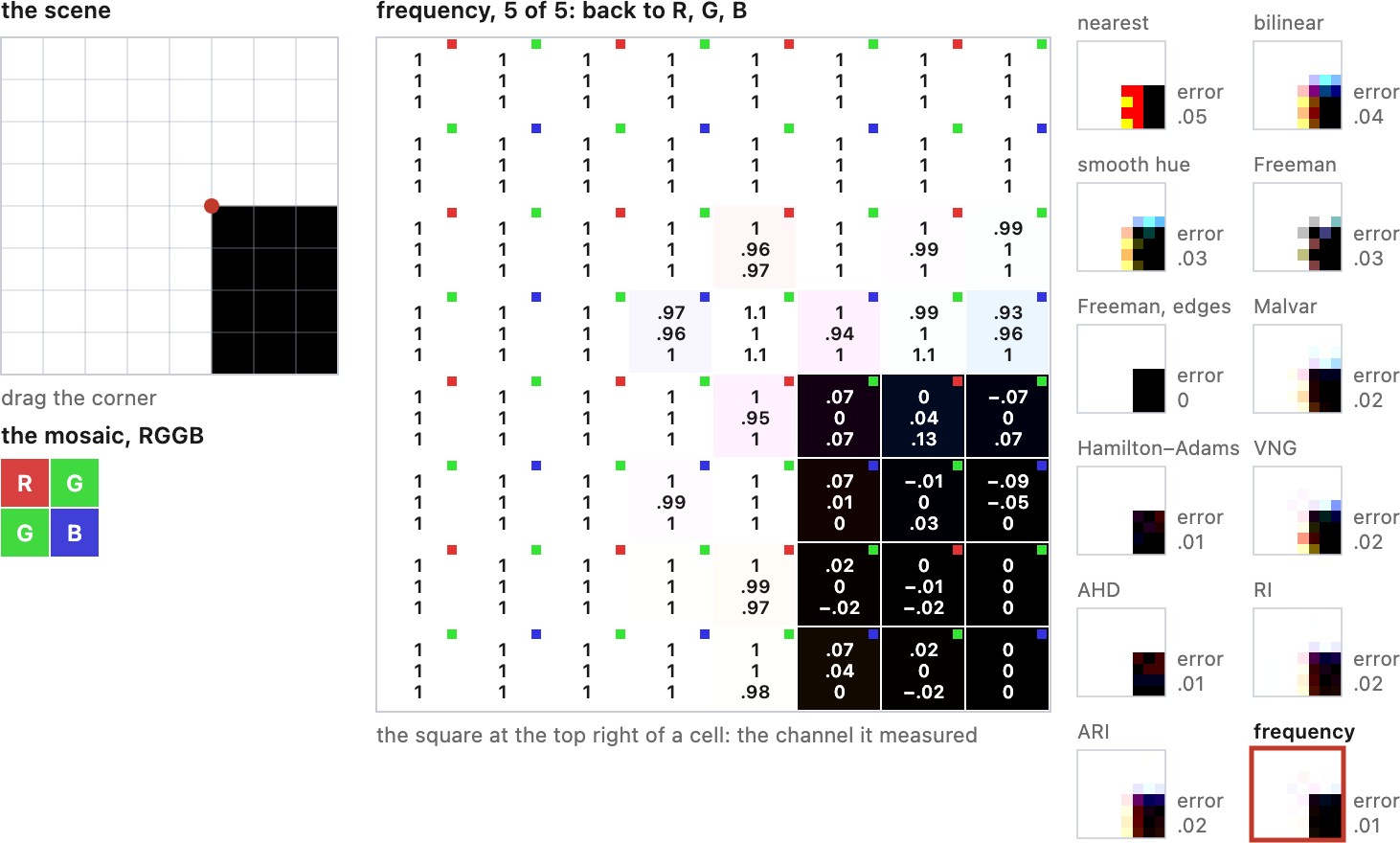
Smooth hue transition Cok 1987 (smooth hue transition), one of the first methods to use one channel to reconstruct another, interpolates green first and then interpolates hue rather than red and blue: the ratio $R/G$ at the red sites, spread to its neighbors and multiplied back by green. It assumes that hue changes slowly across an object even where brightness does not. The choice of hue coordinate matters, and the lab lets you switch it: a ratio becomes unstable where green is near zero, a difference $R-G$ does not, and a log ratio sits in between. The difference form is the recipe of Interpolate differences, not channels.

Its three steps are the smooth-hue stages of Figure 15.2.2⛶ fullscreen.

Freeman's method Freeman 1988 (median demosaicking) demosaicks with bilinear interpolation, then cleans up the hue: it applies a 3 × 3 median to the difference channels $R-G$ and $B-G$ and adds green back. Within an object the color difference is nearly constant, so a false-color pixel is an isolated outlier in a flat channel, which is exactly what a median removes. A 5 × 5 median often does a better job, because false color on fine texture tends to come in clusters wider than a 3 × 3 window can outvote, though a larger median also starts to carry color across object boundaries. The median does nothing for zippering in the green channel, so although the method is described on top of bilinear, it is mostly used as a clean-up step on top of a better demosaicker. Figure 15.2.1⛶ fullscreen offers both bases: on bilinear, the median removes most of the fringes and leaves the zippering; on the chapter's edge-based demosaicking, the green is already good and the median only has the remaining false color to remove. The same pass survives as the final clean-up of many later methods, AHD among them. (Freeman's patent differs in its details: it describes two colors alternating along a line, interpolates each linearly, and applies a one-dimensional median to their difference, five pixels wide in its example, with each pixel keeping its own measured value. The two-dimensional Bayer version above is the one usually implemented.)

Figure 15.2.2⛶ fullscreen shows the three steps on the grid.

Gradient-corrected linear interpolation Malvar et al. 2004, by Malvar, He and Cutler, keeps a fixed linear filter but adds the Laplacian of the channel measured at the center pixel, scaled by a gain, to the bilinear estimate of each missing channel. A red pixel's curvature, for example, corrects the green estimated there, on the assumption that the channels vary together. The result is a set of fixed 5 × 5 filters with no decisions, so it is fast, easy to run on a GPU, and free of the unstable direction choices that make mazes; it is, for example, what MATLAB's demosaic function implements. Because it does not adapt, it still blurs across edges where an adaptive method would not.

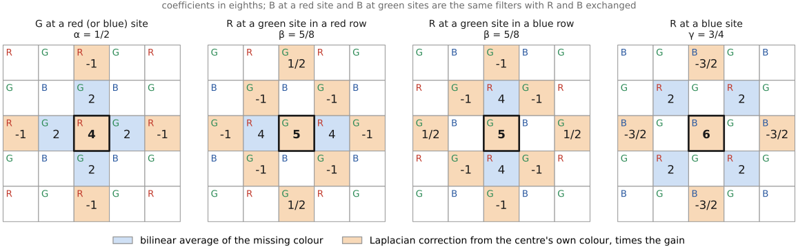
The same correction, pixel by pixel, is in Figure 15.2.2⛶ fullscreen.

Hamilton–Adams Hamilton & Adams 1997, met in Interpolate along the edge, not across it, combines both ideas of the basic chapter, and it does so in three passes over the mosaic, each using the channels already filled in.

1. Green at the red and blue sites. Measure a horizontal and a vertical activity at the site, each the sum of a green gradient across the site and the second difference of the center color along the same line. Interpolate green along the less active direction, as the average of its two green neighbors plus a quarter of the center color's second difference, and use all four neighbors when the two activities are equal. This is the pseudocode of Interpolate along the edge, not across it.
2. Red and blue at the green sites. Now that green exists everywhere, a missing red at a green site is the average of its two red neighbors, horizontal or vertical depending on the row, corrected by half of green's second difference along that line. It is color-difference interpolation in disguise: the result equals the site's green plus the average of the two neighbors' $R-G$, up to the correction.
3. Red at the blue sites, and blue at the red sites. The four nearest samples of the missing color sit on the diagonals, so the method chooses between the two diagonals with the same kind of test, a gradient of the missing color along the diagonal plus green's second difference along it, and interpolates along the calmer one with the same half-weight correction.

# Hamilton-Adams, steps 2 and 3 (step 1, green, is in the edge-directed section)
# step 2: red at a green site in a red row (blue rows: use the vertical pair)
R[x,y] = (R[x-1,y] + R[x+1,y])/2 + (2*G[x,y] - G[x-1,y] - G[x+1,y])/2

# step 3: red at a blue site, choosing a diagonal
dN = abs(R[x-1,y-1] - R[x+1,y+1]) + abs(2*G[x,y] - G[x-1,y-1] - G[x+1,y+1])   # NW-SE
dP = abs(R[x+1,y-1] - R[x-1,y+1]) + abs(2*G[x,y] - G[x+1,y-1] - G[x-1,y+1])   # NE-SW
if   dN < dP: R[x,y] = (R[x-1,y-1] + R[x+1,y+1])/2 + (2*G[x,y] - G[x-1,y-1] - G[x+1,y+1])/2
elif dP < dN: R[x,y] = (R[x+1,y-1] + R[x-1,y+1])/2 + (2*G[x,y] - G[x+1,y-1] - G[x-1,y+1])/2
else:         R[x,y] = (R[x-1,y-1] + R[x+1,y+1] + R[x+1,y-1] + R[x-1,y+1])/4 \
                       + (4*G[x,y] - G[x-1,y-1] - G[x+1,y+1] - G[x+1,y-1] - G[x-1,y+1])/4
# blue at a red site: the same, with R and B exchanged

The corrections are what separate it from bilinear. Each one assumes that the missing channel curves the same way as the channel that was measured or already reconstructed at the site, so a sharp edge in green is copied into red and blue at the same place instead of being smeared into a fringe. The direction tests are what separate it from Malvar–He–Cutler, which applies the same kind of correction everywhere, in every direction. Hamilton–Adams costs a small, fixed amount of work per pixel, and its green step is the starting point of many later methods, including the residual interpolation of the next chapter; its failures are those of any two-way choice: diagonal texture, and fine patterns where both directions look equally active.

Figure 15.2.2⛶ fullscreen runs the three passes on the grid; the grating near 45 degrees shows the failure.

Variable number of gradients Chang, Cheung & Pan 1999 (VNG), VNG, by Chang, Cheung and Pan, replaces the two-way choice with a vote among eight directions, and lets the image decide how many of them to trust. At each pixel it works in the 5 × 5 neighborhood around the site, in four steps.

1. Eight gradients. For each compass direction, north, northeast, east and so on, sum the absolute differences between pairs of same-color samples that lie along that direction on that side of the pixel. Pairing same-color samples keeps the gradient free of the differences between channels. A direction that points into a smooth region gets a small gradient; one that crosses an edge gets a large one.
2. A threshold. From the smallest gradient $g_{\min}$ and the largest $g_{\max}$, set $T = 1.5\,g_{\min} + 0.5\,(g_{\max}-g_{\min})$. The threshold is relative: it asks which directions are nearly as smooth as the smoothest one here, not which are below a fixed number, so the same rule works in shadows and highlights.
3. A vote. Keep every direction whose gradient is below $T$. For each kept direction, average the samples of each color that lie on that side of the pixel, and sum these averages over the kept directions, one sum per color.
4. A color difference. Estimate each missing color from the center sample and the difference of the sums: at a red site, for instance, $\hat G = R + (S_G - S_R)/n$, where $S_G$ and $S_R$ are the sums for green and red over the $n$ kept directions. This is the color-difference idea of Interpolate differences, not channels, averaged over the directions the vote allowed.

# VNG at one pixel, in outline (per-site sample weights omitted)
g = {d: gradient(d) for d in [N, NE, E, SE, S, SW, W, NW]}       # same-color pairs along d
T = 1.5*min(g.values()) + 0.5*(max(g.values()) - min(g.values()))
keep = [d for d in g if g[d] <= T]
S = {c: sum(average_on_side(c, d) for d in keep) for c in [R, G, B]}  # one sum per color
for c in missing_colors:
    value[c] = center_value + (S[c] - S[center_color]) / len(keep)

The number of directions that pass is what gives the method its name and its behavior. In a flat region all eight pass and it averages widely, which suppresses noise; along a straight edge only the two directions parallel to it pass, and it averages along the edge like Hamilton–Adams; at a corner or a line end it can keep three or four, which a two-way choice cannot express (Figure 15.2.4⛶ fullscreen). The cost is about eight gradients per pixel over a 5 × 5 window, several times Hamilton–Adams, and the relative threshold can pass too many directions in fine, low-contrast texture, where everything looks equally smooth. VNG was long one of the modes of the dcraw raw decoder.

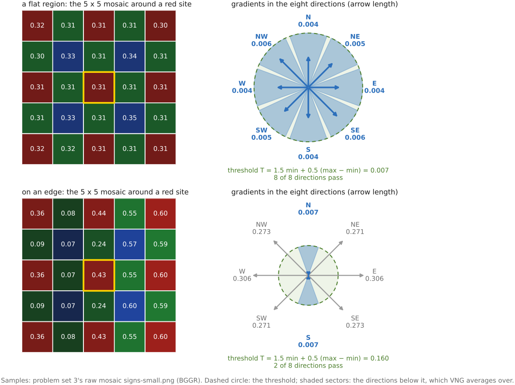
Figure 15.2.2⛶ fullscreen runs VNG on every pixel of the grid.

Two further refinements are common. Iteration: once green and the color differences are in, re-estimate the differences against the interpolated green and repeat. Alternating projections Gunturk, Altunbasak & Mersereau 2002 (alternating projections) formalize this as projecting in turn onto two sets, the images that agree with the measured samples and the images whose red and blue have the same fine detail as green. And directional estimation with explicit noise models: Zhang and Wu's directional linear minimum mean-square-error method Zhang & Wu 2005 (DLMMSE) fuses the horizontal and vertical estimates with weights set by how noisy each one is, rather than choosing one.

Across the eight panes, three things change from method to method. The assumption about images: smooth channels, smooth hue, correlated channels, or edges along one of a few directions. The decision made at each pixel: none for bilinear and Malvar–He–Cutler, a direction for Hamilton–Adams, VNG and AHD (#Adaptive homogeneity-directed demosaicking (AHD), next). And the cost, from nothing for nearest neighbor to two full reconstructions and a color-space conversion for AHD. The residual-interpolation methods (#Residual interpolation and ARI) take the next step by replacing the color difference with the residual of a guided fit.

For reproducible comparisons, state the implementation and demosaicking mode. LibRaw and dcraw expose several algorithms, but their defaults are not interchangeable with the Malvar–He–Cutler method. Compare against a strong classical baseline such as adaptive residual interpolation Monno et al. 2015 (adaptive residual interpolation) as well as a simple linear method.

The sections that follow take up three families that go further: AHD, which builds whole reconstructions in two directions and keeps the more homogeneous one; residual interpolation and ARI, which interpolate what a guided prediction leaves over; and frequency-domain demultiplexing, which treats the mosaic as a modulated signal. The chapter ends with the situations that defeat all of them.

15.2.1 Adaptive homogeneity-directed demosaicking (AHD)🔗⧉

If you want to implement one classical demosaicker that is simple and works well, this is probably your best bet, followed by Freeman's median of the color differences (earlier in this chapter) to remove the false color that remains. Every method so far decides the interpolation direction before interpolating, from gradients in the mosaic. Adaptive homogeneity-directed demosaicking Hirakawa & Parks 2005 (AHD), by Hirakawa and Parks, decides afterward. It reconstructs the whole image twice, once interpolating only horizontally and once only vertically, and at each pixel keeps whichever reconstruction looks more plausible there. The criterion is the key idea: interpolating in the wrong direction averages across an edge and creates colors that exist on neither side of it, so the wrong candidate is less homogeneous, locally, than the right one.

1. Two candidates. Build a full image with every interpolation along rows: green with a Hamilton–Adams-style correction, then red and blue by interpolating color differences. Build a second with every interpolation along columns.
2. A perceptual space. Convert both candidates to CIELAB, so that lightness and color can be compared separately and a distance means roughly what a viewer would notice (Chapter 4.5, Advanced color: opponents, perceptually-uniform, and preferred).
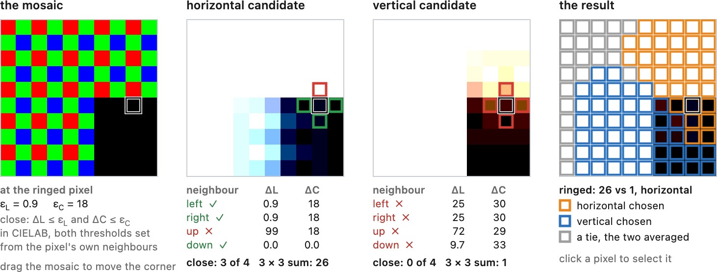
3. Homogeneity. For each pixel of each candidate, count the neighbors in a small window that are close to it in both lightness and color, within thresholds $\varepsilon_L$ and $\varepsilon_C$. The thresholds are set at every pixel from the differences to its nearest neighbors along each candidate's own direction, so the test adapts to local contrast rather than using one number for shadows and highlights.
4. The choice. Sum each candidate's counts over a 3 × 3 window and keep, at each pixel, the candidate with the larger sum; average the two on a tie.
5. Clean-up. Finish with a few passes of a median over the color differences $R-G$ and $B-G$, Freeman's clean-up.

# AHD, in outline
Ih, Iv = demosaic_along_rows(mosaic), demosaic_along_columns(mosaic)
Lh, Lv = to_cielab(Ih), to_cielab(Iv)
eps_L, eps_C = adaptive_thresholds(Lh, Lv)             # per pixel, from nearest-neighbor differences
Hh = count_close_neighbors(Lh, eps_L, eps_C)           # lightness and color both within threshold
Hv = count_close_neighbors(Lv, eps_L, eps_C)
Hh, Hv = box_sum_3x3(Hh), box_sum_3x3(Hv)
out = where(Hh > Hv, Ih, where(Hv > Hh, Iv, (Ih + Iv) / 2))
out = median_color_differences(out, passes=3)

Figure 15.2.5⛶ fullscreen shows the homogeneity test at one pixel.

The figure below runs it on a real facade, where the cornice's horizontal lines choose the horizontal candidate and the window columns the vertical one (Figure 15.2.6⛶ fullscreen), and Figure 15.2.2⛶ fullscreen makes the same choice cell by cell on the chapter's small inputs.

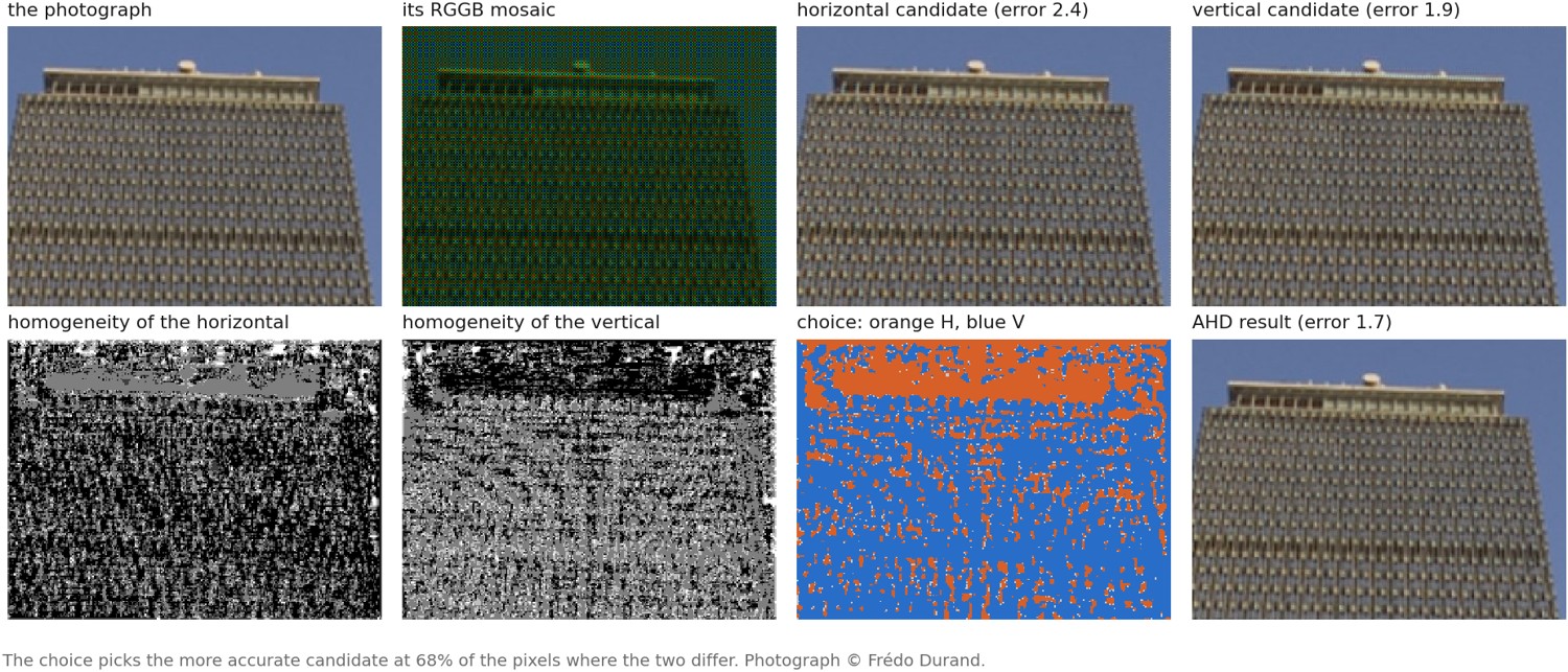
Figure 15.2.2⛶ fullscreen steps through the same algorithm on the small inputs.

AHD costs two full reconstructions, two color-space conversions and the counting, several times Hamilton–Adams. It was the default of the dcraw raw decoder and of many converters built on it for years, and it is still a strong classical baseline. Its limits are the other methods' limits. It still chooses between two directions, so diagonal texture gives both candidates errors and the choice cannot fix them. In fine texture near the sampling limit both candidates are inhomogeneous and the choice becomes erratic, which is where mazes come from. And noise lowers the homogeneity of both candidates everywhere, so the choice degrades as the noise rises, one reason to denoise first or jointly (Chapter 15.8, Joint demosaicking and denoising).

15.2.2 Residual interpolation and ARI🔗⧉

The best-performing classical demosaickers, and the ones to compare against today, come from the residual-interpolation family, and adaptive residual interpolation (ARI) is its strongest member. It appeared a decade after AHD, outperforms it clearly in published comparisons on the standard test sets, and needs no training. It is also built directly on the guided filter of Chapter 10.6, Guided image filtering, so it is a payoff of that chapter rather than a new tool. It takes more work to implement than AHD, which remains the simpler choice when that matters.

The idea changes what gets interpolated. Every classical method interpolates something, and each step of the classical line chose a flatter quantity. Bilinear interpolates the channel itself and fails at edges. Hamilton–Adams and its successors interpolate the color difference $G-R$, which is smooth wherever the two channels differ by an offset, and fails where that assumption does: at a saturated color boundary, at a specular highlight, wherever the ratio between the channels changes rather than their offset. Residual interpolation Kiku et al. 2013 (residual interpolation), by Kiku, Monno, Tanaka and Okutomi, goes one step further. Rather than hope that some quantity is flat, it constructs one: it fits a local prediction of the sparse channel from the dense one and interpolates only what the prediction gets wrong.

Take red, sampled on a quarter of the pixels, and green, already reconstructed everywhere because it is sampled twice as densely. In a small window, model red as a linear function of green,

with $a$ and $b$ estimated from the red samples that exist in that window. This is a guided filter with green as the guide He, Sun & Tang 2013 (guided filter), restricted to the measured sites. In a window $\Omega$, with $\mathcal R$ the set of sites where red was measured, solve

where $\epsilon>0$ stabilizes the slope. Unmeasured sites must not enter the fit as zeros; a window with no red sample has to grow or fall back to a simpler estimate; and since every pixel lies in many windows, the overlapping predictions are averaged, which is the guided filter's own rule. The tentative estimate $\tilde R$ is a full-resolution red built entirely out of green's structure, and it follows a change of contrast between the channels that a difference cannot. The residual is the part of red that green cannot explain,

and the reconstruction interpolates it, by any simple method, and adds it back:

The prediction carries the shared detail, and the residual corrects its errors where measurements constrain them. When the local model explains the structure the channels share, the residual is smaller and flatter than the color difference, and the same cheap interpolator does much less damage to it. That flatness is an assumption to test, not a property the fit enforces: a small residual at the measured sites does not prove that the residual between them is small or smooth, and a misleading guide, a sharp color boundary or a poorly conditioned fit can transfer the wrong structure into the result.

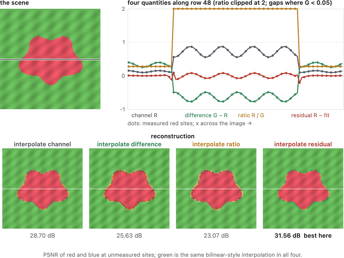
The full algorithm applies the same idea twice, first to green and then to red and blue.

1. Green first. Estimate green along rows and along columns separately, each time guiding by the measured red or blue along that line and interpolating the residual along it, then combine the two directional estimates with weights that favor the direction whose color differences vary less locally.
2. Tentative red. With the full green as the guide, fit a local linear model $\tilde R = aG + b$ in each window, using only the sites where red was measured, and evaluate it everywhere.
3. Residual. At the measured red sites, form $R-\tilde R$.
4. Interpolate and add back. Interpolate the residual bilinearly to every site and add it to $\tilde R$. Blue is the same with blue's samples.

On a red flower against green leaves, the residual is close to zero where the color difference is large, and residual interpolation scores 3.3 dB above AHD (Figure 15.2.8⛶ fullscreen).

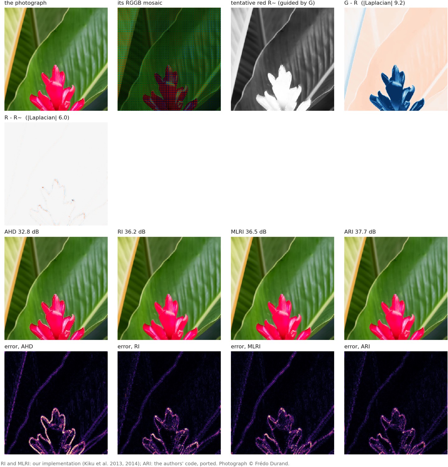
Minimized-Laplacian residual interpolation, MLRI Kiku et al. 2014 (minimized-Laplacian residual interpolation), changes only how $a$ and $b$ are fitted: instead of least squares on the values, it minimizes the Laplacian energy of the residual, which is what the final bilinear interpolation needs to be small. It changes how the regression coefficients are estimated, not which channel serves as the guide. ARI Monno et al. 2015 (adaptive residual interpolation), by Monno, Kiku, Tanaka and Okutomi, iterates both, using each output as the next guide, and at each pixel selects the variant and the number of iterations whose residual is smoothest, judged by the local fit. That is the direction-selection idea of Hamilton–Adams operating one level up: not which direction to interpolate in, but which method to trust here. A later version extends it to multispectral filter arrays Monno et al. 2017 (ARI, multispectral). The authors' reference code has been used widely enough in later work that comparisons against it can be trusted.

# Residual interpolation for red, green already reconstructed (blue is the same)
def residual_interpolation(G, R_mosaic, red_mask, radius, eps):
    a, b = masked_guided_fit(guide=G, target=R_mosaic, mask=red_mask, radius=radius, eps=eps)
    R_tent = box_mean(a, radius) * G + box_mean(b, radius)     # guided filter output
    residual = where(red_mask, R_mosaic - R_tent, 0)
    return R_tent + bilinear_from_samples(residual, red_mask)

# MLRI: the same, with a and b fitted to minimize the Laplacian of the residual
# ARI, in outline: at each pixel keep the (method, iteration) whose residual is smoothest
estimates = []
guide = G
for k in range(K):
    for method in [RI, MLRI]:
        R_k = method(guide, R_mosaic, red_mask)
        estimates.append((R_k, laplacian_energy(R_mosaic - R_k, red_mask)))
    guide = R_k
R = per_pixel_argmin(estimates)          # smoothest residual wins, in a local window

Figure 15.2.2⛶ fullscreen steps through residual interpolation cell by cell on the chapter's small inputs, from the directional green to ARI's per-pixel choice, and the demosaicking lab at the start of this chapter (Figure 15.2.1⛶ fullscreen) runs the same code on photographs.

The limits are the guided filter's. A local linear model cannot follow channels that are related nonlinearly, at clipping or under strong chromatic aberration, and fitting $a$ and $b$ from a few noisy samples is unstable, so noise should be removed first, accounted for within the fit, or handled by joint reconstruction (Chapter 15.8, Joint demosaicking and denoising).

This family, not bilinear interpolation, is the baseline a learned demosaicker should be measured against. It embodies three separate decisions: predict one channel from a guide, interpolate what the prediction missed, and choose locally between useful variants. A learned model can change any of the three, and a comparison with bilinear alone leaves those established improvements unaccounted for, so it cannot tell which part of a network's gain required learning. Compare actual accuracy, noise assumptions and runtime; no ranking of classical methods, and no fixed advantage in decibels, carries over across datasets and settings. A network can represent similar cross-channel predictions, but it chooses what to interpolate implicitly, which is one reason it is hard to say what it learned: a benchmark gain does not show that it learned this algorithm, and attributing the gain requires controlled experiments rather than an analogy between architectures (Chapter 15.6, Learned demosaicking).

15.2.3 Demosaicking as demultiplexing: frequency-domain methods🔗⧉

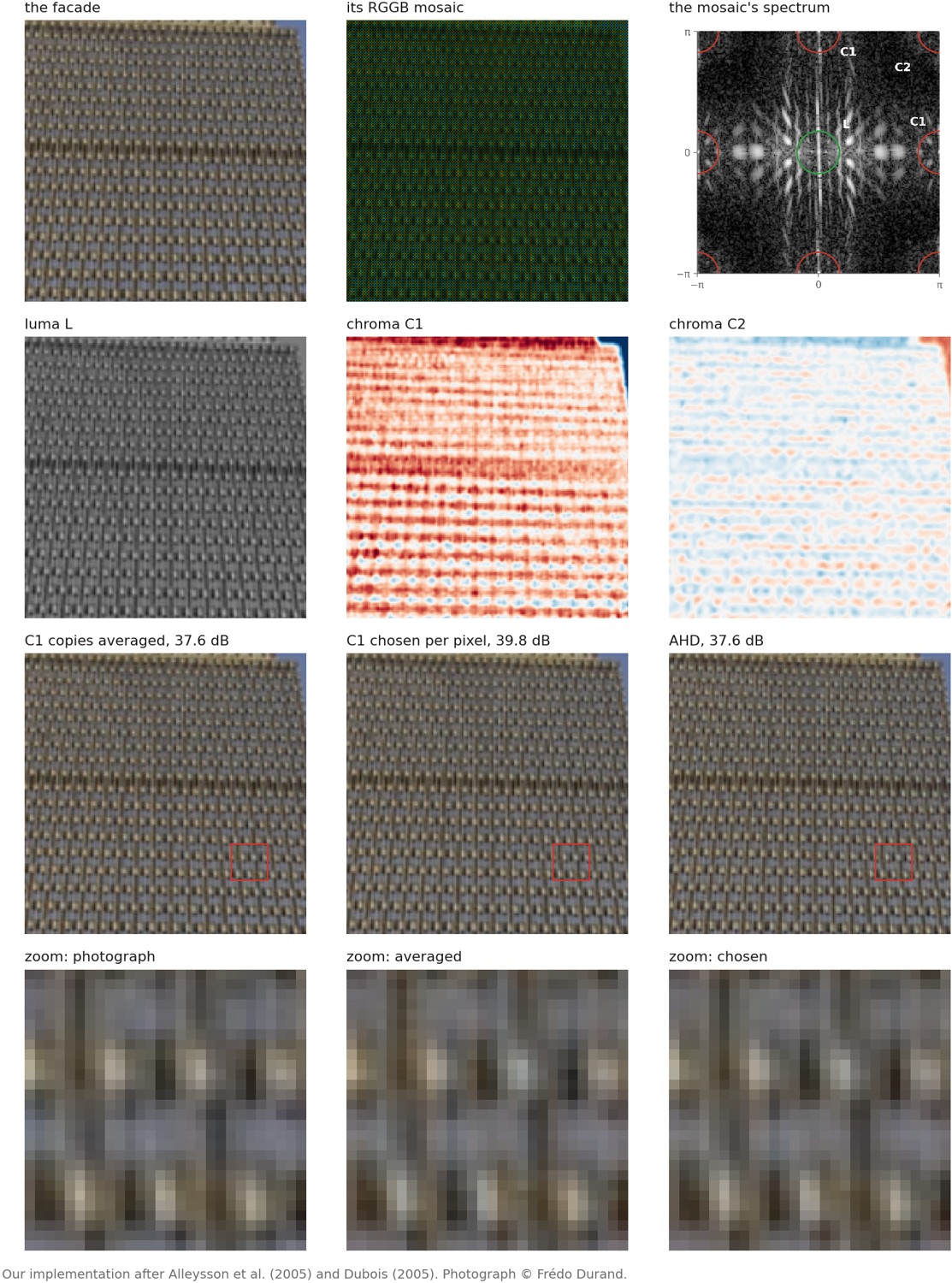
One family of methods treats the mosaic the way a radio engineer treats a signal. As Chapter 15.3, Mosaics and aliasing shows, a Bayer mosaic is exactly a luma component $L$ plus two chroma components modulated onto carriers at the highest frequencies the grid supports: $C_1$ on the horizontal and vertical carriers, $C_2$ on the diagonal one,

Demosaicking is then demultiplexing: isolate each modulated chroma band with a bandpass filter, shift it back to baseband by multiplying by its carrier, and take the luma as what remains. Alleysson, Süsstrunk and Hérault Alleysson, Süsstrunk & Hérault 2005 (frequency-domain demosaicing) arrived at this from the side of human vision, where luma and chroma are carried separately; Dubois Dubois 2005 (frequency-domain demosaicking) made it adaptive. Nowhere else in this chapter is the algorithm itself the frequency argument, rather than a heuristic that happens to be analyzable in frequency terms.

1. Diagonal chroma. Filter the mosaic with a bandpass filter centered on the diagonal carrier and multiply by $(-1)^{i+j}$ to bring $C_2$ back to baseband.
2. Axial chroma, twice. $C_1$ is carried twice, on the horizontal and on the vertical carrier. Extract it from each with its own bandpass filter and demodulate.
3. Choose the cleaner copy. Luma detail leaks into the two copies differently: a vertical texture puts its energy near the horizontal carrier and spoils that copy, while the vertical copy stays clean. Dubois weights the two estimates at each pixel by the local energy of the crosstalk in each, which is the edge-direction idea of this chapter moved into the frequency domain.
4. Luma. Remodulate the chroma estimates and subtract them from the mosaic; what remains is $L$.
5. Back to RGB. $G=L-C_2$, $R=L+C_2+2C_1$, $B=L+C_2-2C_1$.

# frequency-domain demosaicking (Dubois style), for an RGGB mosaic y
C2  = lowpass(bandpass(y, carrier=(pi, pi)) * alternate(i + j))
C1h = lowpass(bandpass(y, carrier=(pi, 0))  * alternate(i))
C1v = lowpass(bandpass(y, carrier=(0, pi))  * alternate(j))
eh, ev = local_energy(crosstalk_h), local_energy(crosstalk_v)   # luma leaking into each copy
C1  = (ev * C1h + eh * C1v) / (eh + ev)                         # trust the cleaner copy
L   = y - C1 * (alternate(i) + alternate(j)) - C2 * alternate(i + j)
G, R, B = L - C2, L + C2 + 2*C1, L + C2 - 2*C1

Figure 15.2.2⛶ fullscreen runs the same demultiplexing on the small inputs.

The filters are where the quality lives. Leung, Jeon and Dubois Leung, Jeon & Dubois 2011 (least-squares luma-chroma demultiplexing) design them by least squares on training images rather than by hand, the least-squares luma-chroma demultiplexing that is the version to cite for performance: a small learned element inside an entirely classical structure. The limit is the one Chapter 15.3, Mosaics and aliasing names: where luma and chroma overlap in frequency, as on fine texture near the carriers, no linear filter can separate them, and the leftover luma shows up as false color.

On the upper floors of a tower facade, where the window grid approaches the carriers, choosing the cleaner copy of $C_1$ per pixel removes much of the false color that averaging the two copies leaves, and the method scores above AHD (Figure 15.2.9⛶ fullscreen). The same implementation falls below bilinear interpolation on the flower of Figure 15.2.8⛶ fullscreen, whose saturated edges carry chroma at frequencies the low-pass filters remove.

15.2.4 Where the classical methods stop🔗⧉

Four situations defeat this family, and they are worth listing because the learned methods of Chapter 15.6, Learned demosaicking are judged on exactly them.

Diagonal edges can challenge a horizontal/vertical decision. More directions or a broader model can help; failure is not inevitable on every diagonal.

Repetitive texture near the sampling limit can alias into apparently consistent false structure. Wider context helps some cases, but a single mosaic may leave genuine ambiguity.

Clipped samples no longer report the incident signal linearly. Mark them and avoid treating their color differences as ordinary measurements. The amount of recoverable highlight color depends on which channels remain useful.

Noise perturbs gradients and can switch interpolation decisions. The error depends on signal-to-noise ratio, not ISO alone. Chapter 15.8, Joint demosaicking and denoising incorporates this uncertainty in reconstruction.