15.0 DEMOSAICKING AND JOINT METHODS⧉
A Bayer sensor measures one color at each photosite. A mosaic of red, green and blue filters sits over the pixels, with green on half of them and red and blue on a quarter each, so each pixel records a single filtered value (Chapter 4.6, Sensing color: multiplexing strategies, Figure 15.0.1). Demosaicking reconstructs the two missing values at every pixel.
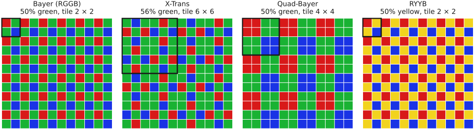
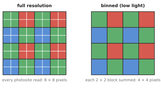
Bayer's is the most common mosaic, not the only one. Fujifilm's X-Trans repeats a 6 × 6 tile with more green than Bayer and at least one pixel of every color in every row and column (Figure 15.0.1). Its less regular layout breaks up the periodic structure that turns fine patterns into color moiré on a Bayer sensor, which lets the cameras that use it leave out an optical low-pass filter, and it needs a demosaicker of its own. Quad-Bayer, common in phone sensors with many small pixels, puts four adjacent pixels under each color filter, a Bayer pattern of 2 × 2 blocks. In low light the sensor combines each block into one larger, less noisy pixel; in good light it reads every pixel and remosaics them into a full-resolution Bayer image (Figure 15.0.2); and the four pixels of a block can be given different exposures to extend dynamic range. Nona-Bayer layouts, Samsung's Nonacell for example, push the same idea to 3 × 3 blocks: a 108-megapixel sensor that bins to 12 megapixels in low light. Other arrays, such as RYYB and RGBW, trade color accuracy for light. Chapter 15.5, Alternative color filter arrays treats these layouts, and Chapter 15.12, Hardware alternatives to the mosaic the sensors that avoid a mosaic altogether.
Demosaicking is one of the fundamentally ill-posed problems of computational photography. We need three numbers per pixel and we have measured one. Many full-color images agree exactly with the same mosaic, and they differ where it matters most, at fine texture and edges, where a wrong choice shows up on fences and fabric as false color, zippering or a maze pattern. Our only hope is to use what we know about natural images, the prior of Chapter 7.1, Imaging as Bayesian inference with probabilistic priors: for example, their color channels share edges, and color varies more slowly than brightness.
This also makes demosaicking hard to measure. On the vast majority of pixels, flat regions, gentle gradients and ordinary edges, almost any reasonable method is nearly exact. The mistakes are rare, but when they happen they are catastrophic and very visible: zippering along an edge, false color on a fence, moiré on fabric, a maze in fine texture. Averaged over a whole image, a few thousand badly wrong pixels among millions barely move a statistic such as mean squared error or PSNR, so two methods can score almost the same while one of them has artifacts that ruin the picture. Demosaickers are therefore judged on the hard cases themselves: error maps, the worst few percent of pixels, and test sets built from the patterns that fail, which is also how the learned methods of Chapter 15.6, Learned demosaicking are trained.
Demosaicking is one of several areas of computational photography, with denoising and super-resolution, where traditional techniques use these regularities implicitly, through the careful design of smart algorithms rather than an explicit model. Interpolating along an edge rather than across it assumes that edges are continuous; interpolating color differences rather than colors assumes that the channels share structure. The field is now changing, from designing algorithms that embody the regularities to learning them from data with deep networks, which can capture regularities no hand-designed rule states. Where each approach runs is set by computation. A camera's image signal processor demosaics every preview and video frame at full resolution in a few milliseconds, so it still runs hand-designed methods of the kind described in Chapter 15.1, Basic traditional demosaicking and Chapter 15.2, Advanced traditional demosaicking. Learned demosaicking has shipped mainly in desktop raw converters, which can spend seconds on one photograph. Phones sit in between: a still photograph gets up to a second or so of processing after the shutter, enough to run networks at full resolution, though manufacturers do not say whether those networks replace the demosaicker, and some phone pipelines avoid single-frame demosaicking by merging a burst of raw frames directly onto a full-color grid.
The part follows that arc. Classical methods rest on two ideas: interpolate along an edge rather than across it, and interpolate a quantity that varies less than the channels themselves, such as the difference between two channels or the residual left after predicting one channel from another Kiku et al. 2013 (residual interpolation). Both assume the channels share structure, which colored edges, clipping and chromatic aberration can violate (Chapter 15.1, Basic traditional demosaicking, Chapter 15.2, Advanced traditional demosaicking). Chapter 15.3, Mosaics and aliasing looks at the mosaics in the Fourier domain, where false color and moiré are aliasing, and at the optical filters that try to prevent it. Chapter 15.4, Optimizing and searching classical demosaickers keeps the hand-made structure and lets data set its constants or search for its structure, Chapter 15.6, Learned demosaicking replaces the rule with a trained one, and Chapter 15.11, Synthetic data, unprocessing, and raw reconstruction asks where the training pairs come from. Demosaicking also interacts with noise: interpolation turns independent sensor errors into correlated color errors, and a denoiser that ignores the mosaic mixes unlike measurements, so Chapter 15.8, Joint demosaicking and denoising and Chapter 15.9, Joint methods and the end-to-end pipeline estimate them together, which helps without automatically beating a well-designed sequence. Chapter 15.10, Quad-Bayer and Nona-Bayer processing covers the grouped layouts of phone sensors, where the industry's remosaicking detour meets learned direct reconstruction. The remaining chapters cover alternative arrays, hardware that avoids the mosaic, and neighboring raw-stage corrections. Throughout, keep the raw measurements and their metadata, the mosaic layout, units, noise and clipping, available to whatever reconstructs the image.
Contents of this part
- 15.1 Basic traditional demosaicking
- 15.2 Advanced traditional demosaicking
- 15.3 Mosaics and aliasing
- 15.3.1 Each channel lives on a sparser lattice
- 15.3.2 All channels at once: luma and chroma
- 15.3.3 False color and moiré as spectral overlap
- 15.3.4 X-Trans, Quad-Bayer and Nona-Bayer in the Fourier domain
- 15.3.5 Prefiltering a mosaic: one blur for three lattices
- 15.3.6 Anti-aliasing filters are disappearing
- 15.3.7 Nano-prisms as anti-aliasing filters
- 15.4 Optimizing and searching classical demosaickers
- 15.5 Alternative color filter arrays
- 15.5.1 Fuji's X-Trans
- 15.5.2 Quad-Bayer and its modes
- 15.5.3 RGBW and sparse color
- 15.5.4 Designing the array and the algorithm together
- 15.6 Learned demosaicking
- 15.7 Neighboring problems in the raw stage
- 15.8 Joint demosaicking and denoising
- 15.9 Joint methods and the end-to-end pipeline
- 15.10 Quad-Bayer and Nona-Bayer processing
- 15.11 Synthetic data, unprocessing, and raw reconstruction
- 15.12 Hardware alternatives to the mosaic
- 15.12.1 Pixel shift: spending time, precisely
- 15.12.2 Foveon and stacked photodiodes: spending silicon depth
- 15.12.3 Assorted pixels: spending spatial resolution on another axis
- 15.12.4 RGB-NIR: adding a band the eye does not have
- 15.12.5 Color wheels: spending time, sequentially, for many bands
- 15.12.6 Four ways to multiplex color
- 15.12.7 Routing color instead of filtering it
- 15.12.8 One table, one question
- 15.13 Demosaicking TLDR