14.7 Generative super-resolution🔗⧉

A highly enlarged patch can admit several plausible textures. Conditional generation models such alternatives given the measurement, rather than returning only one point estimate. Practical diffusion models approximate a learned conditional distribution; it need not equal the real camera posterior.

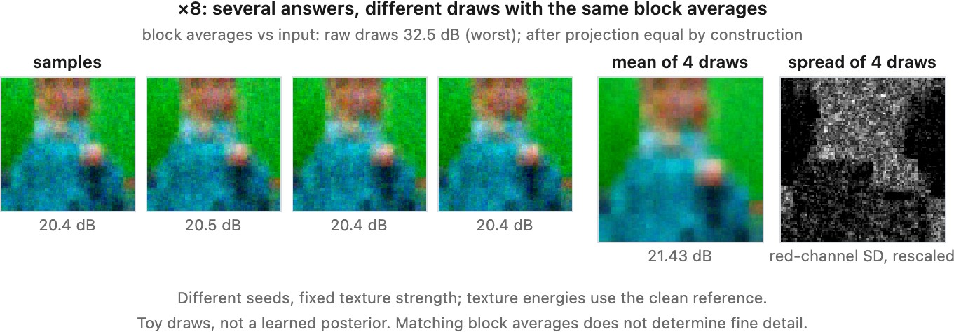
Repeated samples can reveal some of the model's alternatives. They are still estimates, and their variability is not automatically calibrated uncertainty about the scene.

14.7.1 Conditional generation🔗⧉

A diffusion model generates by starting from noise and denoising repeatedly at decreasing noise levels. To make it produce an image consistent with a measurement, the process has to be conditioned on $y$, and there are two families of answer.

Train it in. Give the network the low-resolution image as an extra input, upsampled to the target size, and train on pairs. SR3 (Saharia et al. 2022 (SR3)) does this, and the result is a model that only does super-resolution, at the scale factor and degradation it was trained for. StableSR (Wang et al. 2024 (StableSR)) and DiffBIR (Lin et al. 2024 (DiffBIR)) do the same thing on top of a large pretrained image model, adapting it with a conditioning branch rather than training from scratch, which is what makes the prior strong enough to be interesting at high scale factors.

Steer at sampling time. Keep an unconditional model and modify each step so that the sample moves toward consistency with $y$. The clean version of this is to add the gradient of the data term to the score at every step,

which is Bayes' rule differentiated for the clean-image variable. At a noisy diffusion state, the relevant likelihood is conditioned on that state and integrates over possible clean images; substituting the noisy state into $p(y\mid x)$ generally gives a different quantity. Diffusion posterior sampling (Chung et al. 2023 (DPS)) and DDRM (Kawar et al. 2022 (DDRM)) are two ways of making that practical. The appeal is that one trained model serves every inverse problem, which is exactly the plug-and-play argument of Chapter 13.11, Denoising as a universal prior with sampling in place of optimization.

For Gaussian measurement noise, a common guidance approximation differentiates a residual through a clean-image prediction $\hat x_0(z_t)$:

The Jacobian propagates the measurement error back to the diffusion state. Omitting it is another approximation, not the exact chain rule. A sampler must use its own state parameterization, time schedule, guidance rule and treatment of capture noise. DDRM and diffusion posterior sampling are distinct algorithms; combining an arbitrary denoiser score, this gradient and a DDIM update is not a specified implementation of either.

The guidance calculation itself has a short implementation in an automatic-differentiation system:

# One guidance evaluation, not a complete diffusion sampler.
# clean_prediction uses the model's documented state/time parameterization.
x0 = clean_prediction(z_t, t)
residual = A(x0) - y
loss = squared_norm(residual) / (2 * sigma_n**2)
guidance = -gradient(loss, with_respect_to=z_t)

The derivative must pass through clean_prediction and the forward operator. Detaching x0 from the differentiation graph would eliminate that path. Insert this guidance only through the update rule of the chosen conditional sampler, with its specified scaling; the four lines do not define a reverse-time transition or its noise variance. This calculation supplies the measurement-dependent direction; the sampler determines how that direction changes the next state.

One complete specification is diffusion posterior sampling (Chung et al. 2023 (DPS), its first algorithm) on a DDPM noise schedule, with a network that predicts the noise added at each step. Every quantity below follows that one convention:

# Diffusion posterior sampling with a DDPM schedule and a noise-predicting network.
# beta[i] is the schedule, alpha[i] = 1 - beta[i], alpha_bar[i] = product of alpha[0..i],
# and alpha_bar[-1] = 1 by convention. A is the forward operator (blur then downsample).
z = standard_normal(image_shape)                      # the state at the final step, N - 1
for i in N-1 down to 0:
    eps = eps_model(z, i)                             # predicted noise in the current state
    x0  = (z - sqrt(1 - alpha_bar[i]) * eps) / sqrt(alpha_bar[i])   # clean prediction
    # unconditional ancestral step from state i to state i-1
    mean = (sqrt(alpha[i]) * (1 - alpha_bar[i-1]) * z
            + sqrt(alpha_bar[i-1]) * beta[i] * x0) / (1 - alpha_bar[i])
    z_next = mean + sqrt(beta[i]) * standard_normal(image_shape) if i > 0 else mean
    # measurement guidance, differentiated through x0 and the network back to z
    residual = y - A(x0)
    grad = gradient(squared_norm(residual), with_respect_to=z)
    z = z_next - (zeta / norm(residual)) * grad
return x0

Each step makes the ordinary unconditional move, then corrects it by the gradient of the measurement residual. The residual is measured on the clean prediction, not on the noisy state, and the gradient flows back through the network, which is the Jacobian term above. Dividing the step size zeta by the residual norm is the step rule of the published algorithm; it keeps the correction from overwhelming the prior early, when the prediction is poor, and from vanishing late. The loop costs one network evaluation and one backpropagation through it per step, about twice an unconditional sample, and it needs the network's gradients. The result is consistent with $y$ only approximately, to a degree set by zeta and the number of steps, which is one reason #Consistency, faithfulness, and what to report measures consistency rather than assuming it.

14.7.2 Sampling against averaging🔗⧉

Under squared error, a conditional mean minimizes expected error; a sample represents one alternative. Means can smooth uncertain detail, while samples may be sharp, smooth or implausible depending on the model and data.

Uncertainty depends on the observation and prior, not only on the scale factor. A badly blurred twofold input can be more ambiguous than a clean repeated pattern enlarged eightfold. A model can also produce nearly identical outputs because it misses alternative explanations.

Compare multiple samples when the sampler is stochastic. Disagreement identifies model variation; agreement does not prove that the measurement determined the answer. Report the weights, seed, sampler and sample-selection policy. Selecting the best sample against the test reference is an oracle evaluation.

Chapter 14.10, Video super-resolution and practical systems discusses deployment constraints, including latency and temporal consistency. A single-step distilled model has different sampling behavior from a long iterative diffusion sampler.

14.7.3 Consistency, faithfulness, and what to report🔗⧉

Three properties get confused in this literature and they are worth separating.

Consistency asks whether $A\hat x$ agrees with $y$ within the capture noise and model error. A nonzero residual is expected in noisy reconstruction. Exact projection can overfit noise; disagreement can reflect an inaccurate forward model rather than a defective network.

Faithfulness asks whether the reconstruction matches the scene. A posterior-mean estimator minimizes expected squared error under its assumed model, but an individual sample can be closer to an individual reference. Practical trained networks need empirical comparison.

Realism concerns appearance and image statistics. A perceptual metric measures only the properties encoded in that metric; it does not prove that outputs follow the true photograph distribution.

Report fidelity, appearance, input consistency and computation separately. PSNR remains informative when interpreted as reference error rather than a complete ranking.

14.7.4 The circle closes🔗⧉

Tweedie's formula Efron 2011 (Tweedie’s formula) relates an exact Gaussian posterior-mean denoiser to the score of the corresponding noisy distribution (Chapter 13.11, Denoising as a universal prior). Plug-and-play optimization and conditional diffusion can reuse related image models, but have different updates, assumptions and convergence questions. Neither algorithm is obtained from the other merely by adding random noise.

This reuse of an image model explains the order of the two parts. Denoising provides a tractable setting in which to learn or derive an image prior. Super-resolution then adds a measurement operator with missing spatial information, making the effect of that prior easier to see. An optimizer seeks a chosen estimate, whereas a conditional sampler can explore alternatives. Their common image knowledge does not remove the difference between those questions.