13.12 Measuring a denoiser⧉
A denoising comparison must state what each method receives and what its output is meant to preserve. Known-level Gaussian denoising, blind raw denoising, and restoration of processed photographs test different capabilities. A burst method also receives more captured data than a single-image method. Scores are useful when these conditions are explicit.
Chapter 9.3, Image metrics develops general image-quality measures. For denoising, the additional tasks are separating residual noise from detail loss, checking the reference, and testing the camera and processing conditions under which the method will be used.
13.12.1 The reference metrics, and what each rewards⧉
For $M$ evaluated scalar samples, recall
The peak $L$ must match the declared intensity range, such as 1 or 255. For one image, higher PSNR means lower MSE. Across images, averaging PSNR is not the same as computing PSNR from average MSE because the logarithm is nonlinear. State which aggregation is used. The posterior mean minimizes expected squared error; this does not prove that it maximizes every expected-log-score objective.
Uncertain edge positions or textures can average into a smooth conditional mean, as Chapter 13.9, Generative denoising with diffusion models explains. Arbitrary extra smoothing can instead increase MSE by removing well-supported detail. PSNR rewards numerical fidelity, not smoothing by itself.
SSIM compares local luminance, contrast, and structure (Wang et al. 2004). LPIPS measures differences between deep features (Zhang et al. 2018); DISTS combines structure and texture similarity in a learned-feature representation (Ding et al. 2020 (DISTS)). They capture aspects of perceptual similarity that pixel error misses, but their agreement with viewers depends on the content and distortion. Report the implementation, input normalization, and model version. A feature-distance score is not proof that a reconstructed detail existed in the scene.
NIQE uses natural-image statistics without a clean reference (Mittal, Soundararajan & Bovik 2013 (NIQE)). Other no-reference metrics use different features and training targets. Their scores measure compatibility with those models, not error against the unknown scene. Blinded human comparison, residual inspection, and repeat-capture measurements are also available without an exact reference. For video, add temporal diagnostics and playback rather than relying on framewise averages.
13.12.2 Comparing operating points⧉
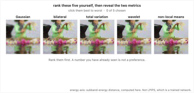
A strength parameter trades residual noise against detail. Sweep it when comparing that tradeoff, or choose settings by a declared validation procedure before examining the test results. Equal numerical parameters across methods do not imply equal strength. A fixed network may offer no useful strength control at all.
One controlled experiment matches output variability in a known flat region, then compares edges and textures. Repeat captures make that variability easier to separate from shading and pattern noise. On a single image, a flat-patch estimate can include real texture, and output variance alone does not measure bias. A method can flatten the patch while changing its mean. Report both when a reference is available.
Inspect the removed residual $r=y-\hat x$ at a fixed display gain. Recognizable structure indicates that the denoiser changed that structure and warrants comparison with the reference or other captures. Even an optimal estimator can leave structure in this residual and noise in its output. A visually noise-like residual is a useful diagnostic, not a necessary and sufficient test of correctness.
13.12.3 What to hold fixed⧉
Use a common protocol for all methods:
- Specify the noise model, level and units, clipping, quantization, and whether the level is supplied or estimated. Reuse the same noisy realization across methods, then repeat over seeds if measuring synthetic-noise variability.
- Specify raw or processed input, channel order, black/white levels, color conversion, tone curve, and the domain in which the score is computed. Raw-domain error and displayed-image error answer different questions.
- Fix the evaluation crop, boundary exclusion, valid-pixel mask, and metric implementation. Record every registration or intensity adjustment made to the reference. Fix these independently of the tested outputs; fitting a different alignment to each output can hide geometric errors.
- Separate training, validation, and test scenes. Crops from the same photograph or frames from one burst should not cross these splits when claiming scene generalization. Choose checkpoints and parameters without test references.
- Match the generalization test to the claim. Hold out cameras for cross-camera performance; for a camera-specific model, hold out scenes and test the relevant exposure, temperature, and processing conditions.
An averaged reference still contains noise and may contain registration artifacts. Under independent, zero-mean reference error $e_r$, measured squared error against $x+e_r$ includes its variance. If the reference shares input frames with the method, the cross term need not vanish and can favor methods that retain shared noise. Keep input and reference captures separate where practical and document residual reference uncertainty.
13.12.4 Ablations, cost, and what to report⧉
An ablation changes one component while preserving the comparison protocol: remove BM3D's second pass Dabov et al. 2007, replace a learned fusion rule with an average, or train a video model without its temporal loss. Retraining may be necessary to distinguish the value of a component from the damage caused by removing it from an already trained system. Report interactions when two components depend on one another.
Measure latency and peak memory at a specified resolution, batch size, numeric precision, hardware, and implementation. GPU timings need synchronization; state whether transfer, model loading, and warm-up are included. Report iteration or sampling counts. For mobile use, energy and sustained throughput can matter alongside single-run latency. For bursts and centered video windows, add capture delay and the number of input frames separately from processing time.
Quality-versus-cost curves expose choices that one default setting hides. Compare actual implementations rather than assigning an intrinsic speed to a method family. A pretrained network needs model weights at inference, not a new training set for every user. Additional frames are also a resource, even if their arithmetic average is fast to compute.
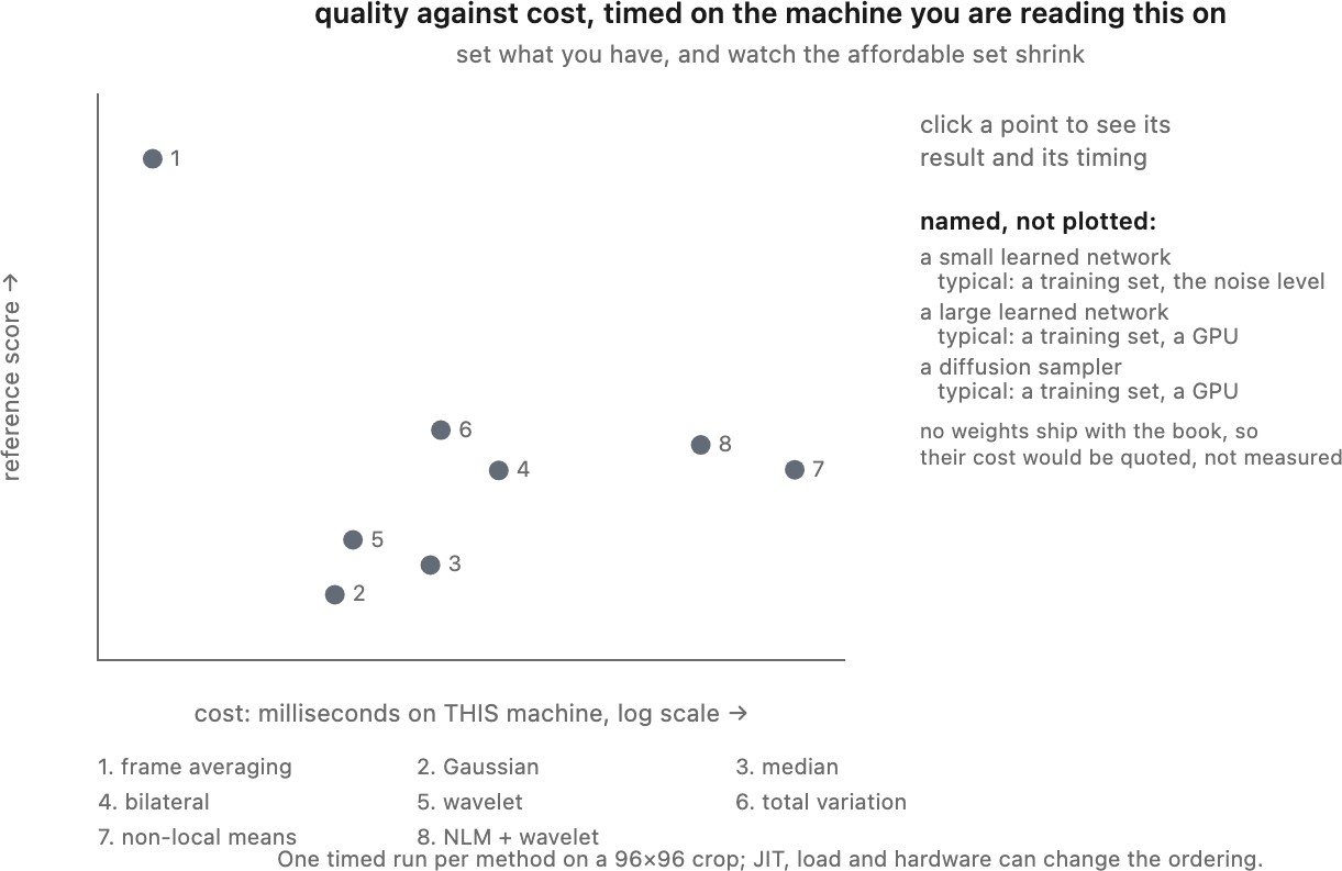
A useful report includes the protocol, quality measures, representative outputs and residuals, component comparisons, and measured cost. Report variation across scenes as well as an average. When estimating uncertainty in the average, resample independent scenes or capture groups rather than treating correlated pixels or overlapping crops as independent trials. Small score differences deserve that context.
13.12.5 The question a benchmark does not answer⧉
SIDD Abdelhamed, Lin & Brown 2018 (SIDD) and DND Plötz & Roth 2017 (DND) provide defined real-camera tests, described in Chapter 13.1, Noise models, transforms, and benchmarks. A score on them establishes performance under their data and evaluation protocol. It does not directly answer how a denoiser will behave after a different camera pipeline, on a new sensor, or with subjects absent from the benchmark.
Build a representative held-out collection for the intended use: dark and bright regions, fine texture, small isolated features, motion where relevant, and the exposure settings actually used. Capture references when feasible, and retain difficult examples that have no reliable reference for blinded visual evaluation. Reference preparation and alignment may require substantial work. A small local collection complements a public benchmark, but cannot by itself establish general performance across all scenes.