13.11 Denoising as a universal prior⧉
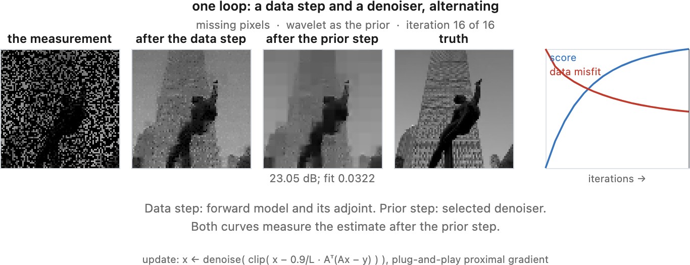
A denoiser encodes regularities of images through its response to a perturbed input. Those regularities can also help reconstruct a blurred image or fill missing samples. Plug-and-play restoration reuses the denoising operation inside an inverse-problem solver, separating it from the measurement model.
There are several mathematical interpretations of this reuse. A proximal denoiser corresponds to an explicit penalty. A posterior-mean Gaussian denoiser determines a score through Tweedie's formula. A general trained network may satisfy neither identity exactly and still be useful in an iterative reconstruction. Keeping these cases distinct explains both the flexibility and the limits of denoiser priors.
13.11.1 Plug-and-play: a denoiser inside ADMM⧉
For measurements $y=Ax+n$ with white Gaussian noise of standard deviation $\sigma_n$, consider
Introduce an image copy $z$ constrained to equal $x$. Scaled ADMM Boyd et al. 2011 (ADMM), with penalty $\mu>0$ and dual variable $u$, gives
The $z$ step is $\operatorname{prox}_{(\lambda/\mu)R}(x^{k+1}+u^k)$. Define a proximal denoiser by
Then $\tau=\sqrt{\lambda/\mu}$ reproduces that step. This is a MAP denoising subproblem for prior proportional to $e^{-R(z)}$, when that prior is well defined. The artificial level $\tau$ differs from the capture noise $\sigma_n$.
Plug-and-play replaces this proximal map by an available denoiser (Venkatakrishnan et al. 2013). The algorithm can be written without evaluating $R$:
z = initial_image(y)
u = zeros_like(z)
for k in 0..K-1:                           # fixed mu in this version
    x = solve((A_adjoint A)/sigma_n**2 + mu*I,
              A_adjoint(y)/sigma_n**2 + mu*(z-u))
    z_new = denoise(x+u, level=sqrt(lambda/mu))
    u = u + x - z_new
    z = z_new
return z
The linear solve uses the exact adjoint and boundary conditions of $A$. The image-copy split differs from the gradient split used for TV. Half-quadratic splitting (HQS) Geman & Yang 1995 (half-quadratic) omits the dual update and alternates a quadratic data step with denoising; at finite penalty, it is not the same algorithm as ADMM.
If the inserted denoiser is not an appropriate proximal map, the original objective and standard convex-ADMM guarantee no longer follow. Convergence can instead be studied under assumptions on the denoising operator and penalty schedule (Chan, Wang & Elgendy 2017 (plug-and-play convergence)). Increasing the penalty alone is not a proof for an arbitrary network. Report data residuals, iterate changes, and the image-copy discrepancy $\lVert x-z\rVert$; stability does not establish reconstruction accuracy.
Read the two updates by their jobs. The data step asks for an image whose simulated measurement agrees with the observation while remaining close to the current auxiliary estimate. The denoising step asks for a plausible image close to its input. Changing the forward operator changes the first problem; reusing a denoiser transfers the second operation across tasks. ADMM also carries a dual variable that coordinates disagreement between the copies. Replacing a true proximal map with an arbitrary denoiser preserves this algorithmic decomposition but does not automatically preserve an objective function or its convergence proof.
13.11.2 Reusing the denoiser across measurement models⧉
For the quadratic data term above, the image update solves
A binary selection mask makes this a pointwise solve: observed pixels combine $y/\sigma_n^2$ with $\mu(z-u)$ and divide by $1/\sigma_n^2+\mu$; unobserved pixels take $z-u$. This also supplies a simple check of the general linear solve. A spatially invariant blur with periodic boundaries can use Fourier diagonalization. More general operators can use iterative linear solvers, as in Chapter 6.9, Efficient linear solvers. Positivity of $\mu$ makes this quadratic system positive definite even when $A$ has a null space.
Changing $A$ adapts the same denoising component to deblurring, subsampling, or missing pixels. This is useful in Chapter 16.2, Non-blind deconvolution, Part 14, Super-resolution and upscaling, and Chapter 21.1, Inpainting, texture synthesis, and object removal. It does not mean that all reconstruction methods in those chapters are plug-and-play. Wiener reconstruction with a Gaussian prior can be solved directly; it is not generally one iteration of the loop above.
Different measurement noise requires a different data term. A raw mosaicked observation and an RGB denoiser also require compatible image variables, color scales, and a forward model that samples those variables correctly. Reusing a natural-photograph denoiser for another imaging modality requires checking its prior assumptions. Better stand-alone denoising scores do not ensure better reconstruction inside every solver.
13.11.3 RED: the denoiser as an explicit regularizer⧉
Regularization by denoising (RED) proposes the functional (Romano et al. 2017)
For differentiable $D$ with Jacobian $J_D$, direct differentiation gives
If $J_D$ is symmetric and local homogeneity implies $J_D(x)x=D(x)$, this simplifies to $x-D(x)$. Under those conditions a descent step on $f+\lambda R_{\mathrm{RED}}$ is
The step size and regularity of the objective still matter for convergence. The residual points opposite to the denoising correction, so subtracting it moves toward the denoised image.
These conditions are restrictive. Reehorst and Schniter (Reehorst & Schniter 2019 (regularization by denoising, clarified)) show that several practical denoisers lack Jacobian symmetry. In that case, using $x-D(x)$ as an update direction need not descend the displayed functional, and a nonsymmetric residual Jacobian prevents interpreting it as the gradient of a smooth scalar potential. A RED fixed-point equation can remain useful without claiming an explicit regularizer:
The corresponding iteration can still be made explicit. This version uses the Gaussian data term defined above:
x = initial_image(y)
for k in 0..K-1:
    data_gradient = A_adjoint(A(x) - y) / sigma_n**2
    denoiser_residual = x - denoise(x, fixed_level)
    x_new = x - step * (data_gradient + lambda * denoiser_residual)
    record(data_residual=A(x_new)-y, iterate_change=x_new-x)
    x = x_new
return x
When the symmetry and homogeneity conditions hold, the expression in parentheses is the gradient of the stated RED objective. Otherwise this is a residual-based iteration aimed at the fixed-point equation, and calling it gradient descent would assert a property the denoiser may not have. This distinction affects which convergence arguments and step-size rules can be used.
13.11.4 Tweedie's formula, and what a denoiser has been computing⧉
Let a clean random image have distribution $p_0$, and corrupt it as $v=x+\tau\varepsilon$, where $\varepsilon\sim\mathcal N(0,I)$ is independent of $x$. The noisy density is
where $\varphi_\tau$ is the Gaussian density with covariance $\tau^2I$. Differentiating the convolution and dividing by $p_\tau(v)$ gives
Thus
This Gaussian identity is commonly called Tweedie's formula (Robbins 1956 (empirical Bayes); Miyasawa 1961; Efron 2011 (Tweedie’s formula)). The score is the gradient of the log noisy density, not of the clean-image density. Its sign corresponds to $D(v)-v$, the negative of the usually displayed removed residual $v-D(v)$.
A network trained with squared error on this Gaussian corruption model estimates the conditional mean at the population optimum and therefore approximates the score. A MAP denoiser, a median estimator, or an arbitrary strong denoiser does not automatically satisfy the identity. Score matching and denoising objectives are related through this Gaussian construction (Hyvärinen 2005 (score matching); Vincent 2011 (denoising autoencoders and score matching)).
For an exact MMSE denoiser, the RED residual is $-\tau^2\nabla\log p_\tau$. This yields a score-based interpretation using the smoothed density even when the local-homogeneity condition needed for the original RED functional does not hold. It does not make the MMSE map identical to the proximal denoiser used in the ADMM derivation.
13.11.5 Sampling with a denoiser-derived score⧉
At a fixed noise level, the score can drive an unadjusted Langevin iteration (Song & Ermon 2019; Kadkhodaie & Simoncelli 2021):
Fresh Gaussian noise distinguishes this sampler from deterministic ascent toward a mode. With an exact score, suitable regularity, small steps, and sufficient mixing, it approximates sampling from $p_\tau$. Finite steps introduce discretization bias. A family of denoisers at descending levels can support annealed sampling or a diffusion reverse process; one arbitrary denoiser called repeatedly is not a complete generative model.
Conditioning generation on a photograph also requires its likelihood, as Chapter 13.9, Generative denoising with diffusion models describes. At nonzero diffusion noise, the likelihood conditioned on the intermediate state is generally not obtained just by substituting that state into the clean-image measurement model. Practical restoration samplers must address or approximate this distinction.
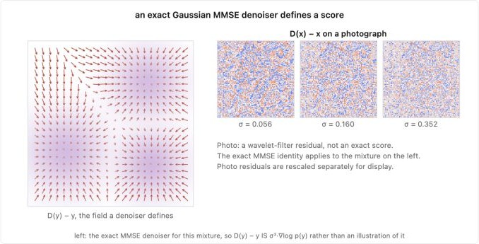
A Gaussian posterior-mean denoiser determines the score of the corresponding noisy-image distribution. This exact identity supports generation; plug-and-play restoration can also reuse denoisers without requiring that identity.
13.11.6 DRUNet as a plug-and-play prior, and continuation⧉
A level-conditioned denoiser lets an outer solver vary the strength of its image prior. In HQS, increasing the quadratic penalty $\mu$ reduces the corresponding denoising level $\sqrt{\lambda/\mu}$. Starting with stronger smoothing and reducing it can help suppress early reconstruction artifacts before retaining finer detail. It is a continuation heuristic, not a guarantee of easier convex subproblems or a globally correct final image.
DRUNet was developed for such reuse in HQS restoration (Zhang et al. 2021 (DRUNet, deep plug-and-play)). Its noise-level input supplies a convenient control, but the model's training range, image scaling, and response to intermediate artifacts still matter. As Chapter 13.7, Learned denoisers notes, its published $L_1$ loss also precludes identifying it automatically with an exact MMSE score estimator.
Specify the schedule, stopping rule, and returned variable when reporting a plug-and-play result. If changing an ADMM penalty, handle the scaled dual variable consistently; the fixed-penalty pseudocode above avoids that additional choice. A continuation schedule in HQS should not be copied into another solver and treated as the same convergence result.
The corresponding HQS implementation is short enough to keep beside the ADMM version. Here the auxiliary estimate has no dual correction, and the specified penalty schedule changes the linear system as well as the denoising strength:
z = initial_image(y)
for mu in positive_penalty_schedule:
    x = solve((A_adjoint A)/sigma_n**2 + mu*I,
              A_adjoint(y)/sigma_n**2 + mu*z)
    z = denoise(x, level=sqrt(lambda/mu))
return z
Keeping both loops visible helps explain what splitting changes. Their data operators are the same, but ADMM carries the disagreement between its two image copies forward through the dual variable. HQS instead relies on the chosen penalty sequence to enforce closer agreement. A finite run must state which copy it returns and how that output agrees with the measurements.
Recap: big lessons of this chapter
A Gaussian posterior-mean denoiser determines the score of the corresponding noisy-image distribution. This exact identity supports generation; plug-and-play restoration can also reuse denoisers without requiring that identity.