13.10 Video denoising🔗⧉

Neighboring video frames often observe the same surfaces with different noise. Combining them can improve quality beyond processing each frame separately, provided that motion, visibility, and changes in appearance are handled. Short exposures, motion blur, occlusion, and low signal still make video denoising difficult.

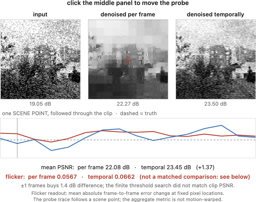
Video also exposes instability that a still image cannot show. A texture may disappear in one frame and return in the next; an edge may change sharpness as its estimated motion changes. Such flicker can be objectionable even when individual frames have small reconstruction errors. Temporal consistency and spatial fidelity therefore need separate inspection.

Track a small patch on a moving sleeve through several frames. The same sensor coordinate sees different material as the sleeve moves; the corresponding scene patch follows a trajectory. Temporal averaging is useful only after identifying that trajectory or an equivalent correspondence. At an occlusion, the sleeve disappears and a background sample is no longer another observation of it. A temporal method must reduce or reject that contribution rather than treating more frames as automatically more evidence. These visibility changes explain why a stable video can require different weights from a collection of independently good still frames.

13.10.1 Temporal redundancy is the resource🔗⧉

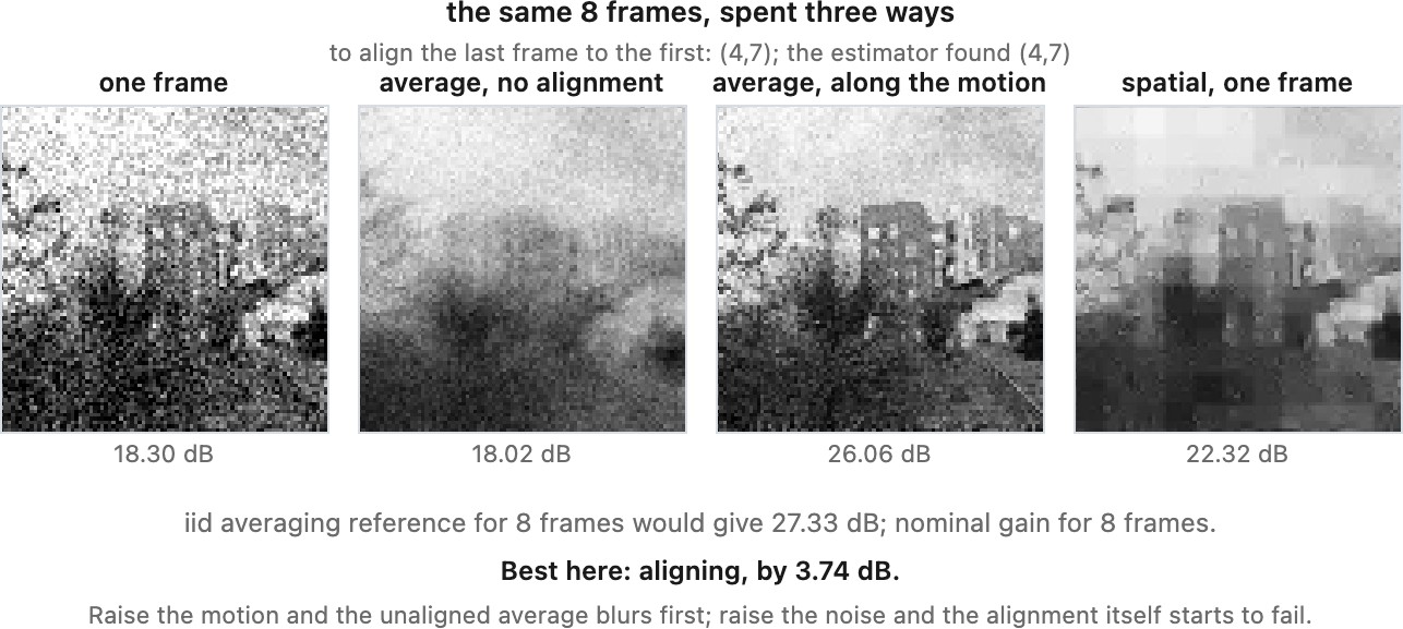
For a static scene with independent, equal-variance frame noise, averaging $N$ frames reduces noise standard deviation from $\sigma$ to $\sigma/\sqrt N$. This is the fixed-per-frame-exposure comparison of Chapter 13.2, Denoising by averaging. It uses $N$ captures; it is not a free gain at fixed total exposure and latency.

To combine moving frames, define $\mathbf d_{t\to s}(p)$ as the displacement from a location $p$ in target frame $t$ to its corresponding location in source frame $s$. Backward sampling then gives

The sampling coordinates point from target to source even though the warped image is described as source-to-target. With nonnegative confidence weights $w_{ts}(p)$, a motion-compensated estimate is

Include the target frame with positive weight so the denominator cannot vanish. Weights can reject occlusions, out-of-bounds samples, and unreliable motion, and can reflect unequal noise variance after exposure normalization. If neighboring frames contribute little, the estimate retains more current-frame noise and may need spatial denoising.

Interpolation changes noise variance and spatial correlation. Flow errors mix scene values, and flow estimated from the same noisy measurements makes the weights data-dependent. The independent-sample formula remains a reference case, not a guarantee for the warped output. Matching pixels across space and time develops correspondence estimation and its failure cases.

13.10.2 Patches in space and time🔗⧉

Searching similar patches across several frames extends the self-similarity idea of Chapter 13.6, Non-local means and BM3D. VBM4D (Maggioni et al. 2012 (VBM4D)) constructs three-dimensional volumes by tracking two-dimensional blocks through time, then groups similar volumes along a fourth dimension. A separable transform exploits spatial structure within blocks, temporal structure along trajectories, and similarity between volumes before shrinkage and aggregation.

VBM4D therefore uses motion trajectories as well as non-local matching; it is not a method that simply avoids alignment. Incorrect trajectories and false matches can damage detail. Matching thresholds, limited groups, and aggregation can reduce their influence but do not make a poor match harmless.

Searching and filtering space-time groups is costly. Window size, frame resolution, implementation, and hardware determine whether a configuration fits a video pipeline. A real-time claim must include those conditions. A causal method uses only present and past frames; a centered window must wait for future frames even if its computation is fast.

13.10.3 Learned video denoisers🔗⧉

A multi-frame network maps a window of observations to a target frame. It can align images or features explicitly, or learn to combine displaced content through its receptive field. Its predecessor from the same authors, DVDnet (Tassano, Delon & Veit 2019 (DVDnet)), aligned neighboring frames with an explicit optical-flow estimate before denoising them. FastDVDnet uses a two-stage cascade on five input frames without an explicit optical-flow stage (Tassano, Delon & Veit 2020 (FastDVDnet)), and the authors report it as much faster than DVDnet at similar quality. This removes the cost and failure modes of a separate flow estimator, while leaving motion handling dependent on the learned model and the size of motion it can accommodate.

Recurrent methods retain a previous output or a hidden feature state. The following illustrates an output-feedback design; other recurrent models propagate features:

state = None
for t, y in frames:
    if state is None or scene_cut(previous_input, y):
        xhat = spatial_denoiser(y, noise_level[t])
    else:
        d = estimate_displacement(target=y, source=previous_input)
        history, valid = sample_source(state, coordinates=grid + d)
        confidence = motion_confidence(previous_input, y, d) * valid
        xhat = fusion_network(y, history, confidence, noise_level[t])
    state = xhat
    previous_input = y
    emit(xhat)

History carries earlier denoising information and earlier errors. Confidence can reduce ghost trails; recurrence alone does not enforce correct temporal behavior. Scene cuts, disocclusions, and large exposure changes require history rejection or reset. Shared state also correlates errors across output frames, so it should not be counted as a growing collection of independent measurements.

Training strategy is a separate choice. Ehret and colleagues adapt a denoiser through frame-to-frame training (Ehret et al. 2019 (model-blind video denoising)); correspondence and the noisy-target assumptions in Chapter 13.8, Denoising without clean data remain central. ViDeNN is a supervised blind video denoiser combining spatial and temporal processing (Claus & van Gemert 2019 (ViDeNN)). Here “blind” means that inference does not require a supplied noise model; it does not mean training without clean targets.

13.10.4 Temporal consistency, and the metric that does not measure it🔗⧉

Framewise PSNR reports average reconstruction error but does not characterize its evolution. Two methods with similar scores can have different flicker, ghosting, and motion detail. View clips at their intended frame rate, including scene cuts and moving fine structures, as well as inspecting still crops.

A simple temporal consistency penalty is

where $m_t$ masks occlusions, invalid warps, and locations where the assumed correspondence is unreliable. Use it only when the denominator is positive. Combine it with a reconstruction term, for example $\mathcal L=\mathcal L_{\mathrm{rec}}+\beta\mathcal L_{\mathrm{temp}}$. Brightness changes and motion-estimation errors can otherwise penalize legitimate changes. A constant output can have excellent temporal consistency and terrible image fidelity, so this loss or metric cannot stand alone. For evaluation, use a common flow/mask protocol rather than letting each method hide its own failures.

Low-light video makes reference capture and alignment particularly difficult. Seeing Motion in the Dark trains on static raw videos with references and adds a temporal-stability objective to support dynamic test scenes (Chen et al., ICCV 2019). This is distinct from the earlier single-image Learning to See in the Dark. Night-mode still photography may accumulate a burst into one photograph; continuous video must produce a stream within its frame-rate and latency constraints.