13.6 Non-local means and BM3D🔗⧉

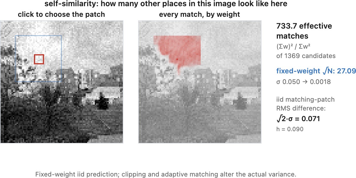
A brick wall supplies many patches with similar mortar lines. Along a straight boundary, neighboring patches contain nearly the same edge. These repetitions let a denoiser use measurements from other parts of one photograph. Non-local means finds them by comparing patches; BM3D also transforms groups of matched patches to separate their common structure from noise.

The connection to Chapter 13.2, Denoising by averaging is useful but conditional. If several locations had exactly the same clean value and independent noise, averaging them would give the familiar variance reduction. Actual patches differ in shading, geometry, and texture, and the algorithm selects them using noisy data. Matching errors introduce bias; overlapping patches and adaptive selection complicate the variance. A match count alone does not predict the denoising gain.

13.6.1 A photograph repeats itself🔗⧉

A single observed value says little about whether two locations depict the same structure. A patch supplies the surrounding edge orientation, texture, and color. Comparing these measurements together makes a match more discriminating, although it cannot prove that two clean patches agree.

Let $P_p y$ extract a patch of $m$ scalar samples around pixel $p$. For distinct patch centers, define the mean squared distance

Under additive independent noise of variance $\sigma^2$, with corresponding samples drawn from distinct pixels,

For two identical, nonoverlapping clean patches under Gaussian noise, the variance of this distance is $8\sigma^4/m$. Larger patches therefore stabilize this particular statistic. Overlap correlates its terms, and a larger patch is less likely to match a genuinely different part of the scene. The formula is not a universal $\sqrt m$ improvement in matching accuracy.

13.6.2 Non-local means: similarity as the weight🔗⧉

Non-local means (Buades et al. 2005) averages observed values with weights derived from patch similarity. One common version compensates for the expected noise contribution:

Here $S_p$ is a bounded search window and $h>0$ has the same intensity units as $\sigma$. The normalization by $m$ in the distance is essential: subtracting $2\sigma^2$ from an unnormalized sum would use the wrong noise scale. The subtraction and truncation are a practical weighting rule, not an unbiased estimator of similarity.

for p in image:
    w = empty_map()
    candidates = search_window(p) excluding p
    for q in candidates:
        d2 = mean((patch(y,p) - patch(y,q))**2)
        w[q] = exp(-max(d2 - 2*sigma**2, 0) / h**2)
    if candidates is empty:
        out[p] = y[p]
        continue
    w[p] = max(w[q] for q in candidates)
    if sum(w.values()) == 0:
        out[p] = y[p]
        continue
    out[p] = sum(w[q]*y[q] for q in candidates plus p) / sum(w.values())

This self-weight convention prevents an exact self-match from overwhelming much smaller neighboring weights. If the candidate set is empty or all weights underflow to zero, return $y_p$. Use a consistent boundary extension when extracting patches. For color images, distances can combine channels and the same weights can filter all channels, with the noise model adjusted for their variances and correlations.

Larger search windows cost more and offer more accidental matches as well as useful ones. Larger $h$ accepts less similar patches and smooths more strongly. Patchwise variants estimate whole patches and aggregate their overlaps. These details distinguish implementations of Chapter 10.2, Non-local means that otherwise share the same equation.

The method also carries a bias. It averages a patch with the patches that resemble it, so it pulls the image slightly toward its own repeated structures, and details with no match elsewhere, a crack in one brick, a single hair, get fewer effective samples and either stay noisy or are smoothed toward their nearest look-alikes. This is the first appearance of a failure mode that every method borrowing evidence from elsewhere in the image shares: good at what repeats, weaker at what does not.

The direct search repeats much of its arithmetic. For a fixed displacement, form an image of squared differences between the input and its shifted copy. A box sum, implemented with a summed-area table Crow 1984 or separable running sums, then gives all patch distances for that displacement. This reduces the cost of comparing large patches. A bounded search window limits the number of displacements; a pilot denoising pass can help select candidates, provided the final average still uses the intended measurements. These accelerations change different parts of the computation and can be combined.

13.6.3 BM3D: group, transform, shrink, aggregate🔗⧉

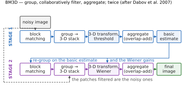
BM3D (Dabov et al. 2007) combines patch matching with Chapter 13.4, Pyramid and wavelet denoising. For each reference patch it selects similar patches, stacks them, applies a transform within each patch and along the stack, shrinks the coefficients, and transforms back. The third dimension indexes patches; it is not a spatial axis in the photograph.

If the patches were identical, an orthonormal transform along the stack with a constant first basis vector would concentrate their shared signal in that component. Real matches differ, so other components also contain signal. Shrinkage can retain these differences when they are sufficiently strong. It can also erase a genuine detail present in only one patch.

The method has two passes. The first uses hard thresholding and aggregates the reconstructed patches into a basic estimate. The second uses that estimate to select groups and estimate coefficient power, but filters groups extracted from the original noisy image. In a simplified orthonormal-transform description, its empirical Wiener gains are

A small pilot coefficient gives a small gain; a large one largely retains the noisy coefficient. With other transform normalizations, replace $\sigma^2$ by the appropriate coefficient noise variance. Group selection and overlapping samples make the actual statistics more complicated than this idealized expression.

basic = aggregate(
    inverse_transform(hard_threshold(transform(group_from(y)), threshold))
    for each reference patch, with group matches found in y)

for each reference patch:
    positions = find_matches(basic)
    c_basic = transform(extract_group(basic, positions))
    c_noisy = transform(extract_group(y, positions))
    gains = abs(c_basic)**2 / (abs(c_basic)**2 + coefficient_noise_variance)
    accumulate(inverse_transform(gains * c_noisy), positions, group_weights)
out = accumulated_values / accumulated_weights

This outlines the data flow; a reproducible implementation must also specify transforms, matching thresholds, group sizes, spatial windows, and aggregation weights. Every reconstructed patch returns to its own original position. Overlapping estimates are combined with spatial and group reliability weights, then normalized. They share input pixels and are not independent new observations.

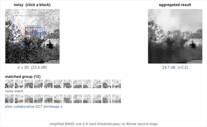
Suppose four matched patches were exactly equal except for independent noise. Along the stack dimension, their common component is constant, while their differences contain only noise. An orthonormal transform separates that constant direction from difference directions. Shrinking the latter suppresses disagreement while retaining the common patch. Real matches are only approximate: a small edge displacement or a texture difference can also occupy a difference direction. BM3D's grouping, shrinkage, and overlap aggregation must therefore balance agreement against genuine variation. This explains why grouping quality matters as much as the transform itself.

13.6.4 The ceiling of hand-designed priors🔗⧉

BM3D remains a useful comparison because it requires a noise level but no learned weights. It can exploit strong repetition within a test photograph even when that photograph differs from a training collection. Irregular fine texture, unique details, and unreliable matching at high noise remain difficult.

Levin, Nadler, Durand, and Freeman (Levin, Nadler, Durand & Freeman 2012) studied denoising limits through statistical models and large collections of natural-image patches. Their analysis relates attainable error to patch size and pixel correlations. Under their model, the best methods of the time were already close to the attainable error for small patches, so further cleverness within a small window had little left to gain, while the bound kept improving as patches grew. Such estimates depend on the image distribution and patch model; they are not a proof that BM3D is optimal or that all hand-designed priors have reached a universal limit. They motivate the use of broader context, which learned methods can exploit without explicitly searching for every matching patch.