12.9 Deep learning approaches to optical flow🔗⧉

Flow networks learn representations and inference rules from examples. Some retain pyramids and warping; others use all-pairs correlations or recurrent refinement. Their relation to classical optimization is useful for explanation, but does not make every architecture an unrolled Horn–Schunck solver Horn & Schunck 1981.

The lineage makes the point concrete. FlowNet (Dosovitskiy et al. 2015) was the proof of concept, the first convolutional network to regress a dense flow field directly, showing the problem was learnable at all (its FlowNet 2.0 successor, Ilg et al. 2017, stacked and refined it into accuracy). PWC-Net (Sun, Yang, Liu and Kautz 2018, at NVIDIA) made the lineage explicit by folding the classical coarse-to-fine pipeline, Pyramid, Warping, and Cost-volume, into one compact, fast network: the same warp-then-refine loop from the last section, now with learned features and a learned per-level update. RAFT (Teed and Deng 2020) is the design that came to dominate: build a four-dimensional all-pairs correlation volume, that is, every pixel's similarity to every other, and apply a recurrent update operator that behaves like an unrolled iterative optimizer refining the field. Finally, transformer flows, FlowFormer (Huang et al. 2022) and GMFlow (Xu et al. 2022), reframe the whole thing as global matching, using attention for cost representation or global correspondence, with different refinement designs. Throughout, the skeleton is the classical one; learning supplies the operators.

12.9.1 The unrolling principle: neuralize the classical solver🔗⧉

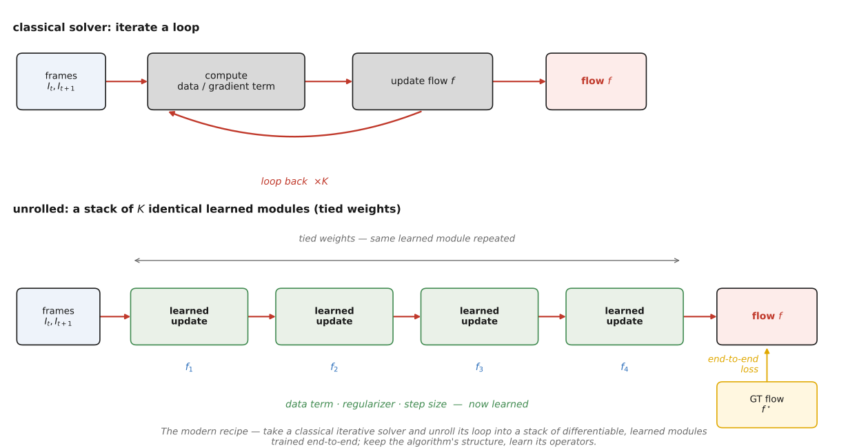
The rest of the section is variations on the same move. A classical flow method iterates an optimizer: compute a data or gradient term from brightness constancy, take a step, repeat until the field settles. Write that step in its plainest form,

where $\mathbf f=(u,v)$ is the flow field, $E$ is the data-plus-smoothness energy of Horn–Schunck, and $\eta$ is a step size. Unrolling takes this loop and straightens it: instead of running an opaque optimizer to convergence, lay out a fixed number of iterations as a stack of differentiable blocks, replace the hand-tuned pieces inside each block, namely the data term, smoothness prior, step size, and coarse-to-fine schedule, with learned operators, and train the entire stack end to end against ground-truth flow. The gradient step becomes a learned update,

This is schematic: a recurrent unit maintains hidden state, consumes context and correlation features, and a prediction head emits a flow increment. It is not simply a stateless GRU-valued gradient. Training does not generally constrain the increment to descend any explicit scalar energy.

The structure supplies a useful inductive bias, while training adapts the features and updates. Its benefit depends on the task and data. Compare accuracy, memory and latency rather than treating one design principle as a guarantee.

12.9.2 Cost volumes and warping inside the net🔗⧉

Two of the classical parts deserve their own look, because they are where matching actually happens inside the network: the cost volume and the warp.

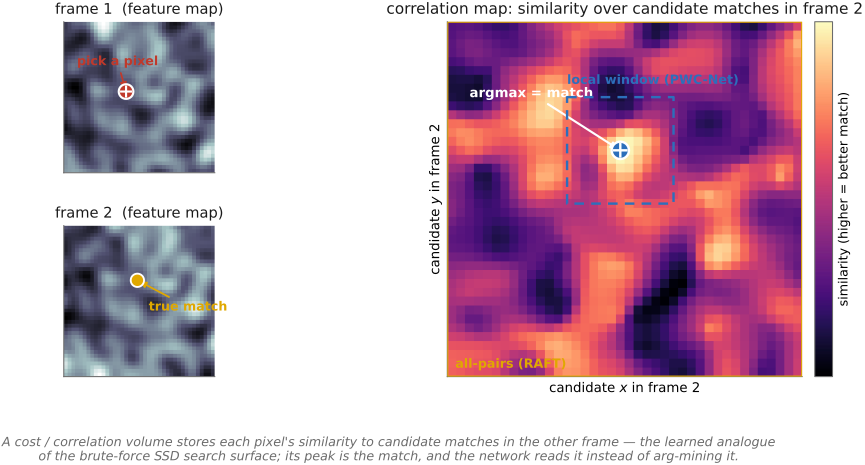
The cost (correlation) volume is the learned analog of the brute-force SSD search surface from Chapter 12.1, Brute force and the classical patch-matching of Chapter 12.8, Optical flow. The classical method, for a pixel in frame 1, scored its sum-of-squared-differences against every candidate offset in frame 2 and took the argmin. The learned version does the same thing on learned features rather than raw RGB: it computes, for each pixel in frame 1, the correlation (a dot product of feature vectors) against candidate pixels in frame 2, over a local neighborhood (PWC-Net) or over all pixels (RAFT's four-dimensional all-pairs volume). The result is a similarity map per pixel whose peak is the match (Figure 2). The decisive difference is what happens next: the classical method arg-mined the surface, committing hard to its peak; the network instead reads the volume: it hands the whole similarity map to the update operator, which can weigh a sharp peak against an ambiguous ridge, fuse it with context, and refine softly. Using learned features here is exactly what lets a match survive the lighting changes and weak texture that break brightness constancy on raw pixels. Flow got the deep-learning treatment relatively late for a clear reason: matching is intrinsically non-local, because a pixel can correspond to anywhere in the other frame, which ordinary convolutions, with their small receptive fields, handle badly. The explicit cost volume is the inductive bias that makes non-local matching tractable, and every method here keeps it in some form.

Warping closes the loop between the volume and the iteration, and it is the move that makes PWC-Net so transparently the classical pipeline. Before correlating at a given pyramid level, PWC-Net warps the frame-2 features toward frame 1 by the current flow estimate, so that only a small residual motion remains to be measured, which means a local cost volume, computed over a tiny neighborhood, suffices. This is precisely the classical coarse-to-fine warp-then-refine loop, now differentiable and living inside the network: align by what you know, measure the leftover, add it back. And the pyramid survives as the network's own multi-scale structure (large motion captured cheaply at the coarse top, refined as you descend), except that the prefilter and the per-level update are learned rather than a fixed Gaussian blur and a fixed least-squares step. PWC-Net is, almost literally, Lucas–Kanade's coarse-to-fine schedule Lucas & Kanade 1981 with every hand-built part swapped for a trained one.

12.9.3 RAFT and the recurrent update🔗⧉

RAFT is the design that came to dominate, and it is best read as the unrolling principle taken to its clean limit (Figure 3). Three classical parts are neuralized and arranged just so. First, learned features: a shared encoder turns both frames into per-pixel feature maps for matching, and a separate context encoder of frame 1 supplies the edge-aware regularization that Horn–Schunck got from a smoothness prior, with the data term and the prior each now learned. Second, an all-pairs correlation volume: RAFT computes the four-dimensional volume of similarities between every pair of feature-grid locations once, up front, and pools it into a small pyramid for cheap multi-scale lookup. Third, a recurrent update operator: a GRU with tied weights that, at each step, looks up correlations around the current flow estimate, combines them with the context features, and emits a refinement $\Delta\mathbf f$, the learned update that stands in for the gradient step, applied over and over to the same shared weights. This is a learned recurrent refinement architecture.

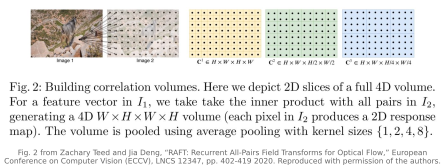
Original RAFT maintains a flow estimate on one feature-grid resolution while pooling the target-coordinate dimensions of its correlation volume for multi-scale lookup. It then upsamples the prediction to image resolution. Shared update weights permit varying the iteration budget, but extra steps do not guarantee monotonic improvement. The explicit all-pairs volume has quadratic storage in the number of feature-grid locations, so resolution and implementation matter.

FlowFormer and GMFlow use attention in different ways [@huang-etal-2022; @xu-etal-2022]. They should not be described as the same one-step replacement for RAFT’s update: cost representation, matching and refinement differ. Compare their actual architectures and evaluation settings before transferring an explanation or speed claim from one to another.

Use the predicted field with the same coordinate, validity and resampling conventions as classical flow. A plausible field in an occluded region remains an inference, not an observed match.

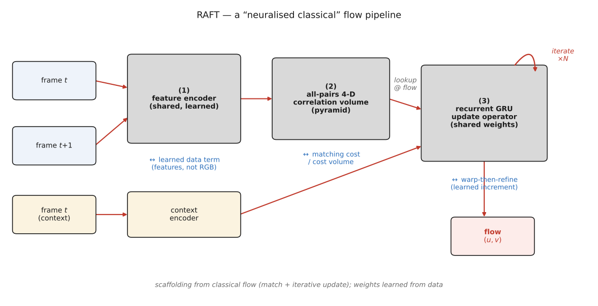
Sharing the update weights makes the refinement loop reusable rather than assigning a different learned module to each iteration. The correlation representation supplies candidate-match evidence, while the current flow estimate determines which evidence the update reads. This separates the evidence from the evolving guess. A larger iteration budget can be tested without constructing a new cascade, but its benefit must be measured. Related correspondence systems reuse this decomposition while changing the geometry or search constraints, as in stereo disparity; they are not automatically identical networks. Downstream, the learned field is consumed the same way a classical one is: to synthesize in-between frames (Chapter 30.4, Frame interpolation and slow-motion synthesis), to estimate and remove camera shake (Chapter 30.6, Video stabilization and rolling-shutter correction), to predict blocks in video coding (Chapter 30.2, Video compression and motion compensation), and to track points over many frames (Chapter 12.4, Feature tracking).