12.8 Optical flow⧉
PS9 (make-your-own) implements Lucas–Kanade optical flow and retiming. → Chapter 1.5, Problem sets (appendix).
You have two consecutive frames of a video, showing a person turning their head, a car crossing the scene, or leaves stirring in the wind, and you want to know, for every single pixel, where it went. Not "the camera panned left" and not "there are three moving objects," but a full, dense field: a little arrow at each pixel saying how far and in what direction that bit of the world slid between the two frames. That field is optical flow, and it is the automatic, dense answer to the same correspondence question Chapter 11.3, Morphing answered by hand. Where morphing made you draw line pairs across two faces, optical flow estimates the entire two-dimensional displacement field straight from the two images, with no human in the loop.
It is also, as we will see almost immediately, a problem that is intrinsically ill-posed, and the derivation makes that explicit. The mathematics will tell us, pixel by pixel, exactly where it cannot recover the motion, and why. That confession is not a weakness to apologize for; it is the most important thing in the chapter, because every flow algorithm ever written is a different answer to the question the math itself raises: given that one pixel can never tell us its full motion, where do we get the missing information?
We pose brightness constancy, linearize it into the optical-flow constraint, one equation per pixel, and immediately hit the aperture problem: one equation, two unknowns. Then come the two classic ways to supply the second equation: Lucas–Kanade (borrow it from your neighbors) and Horn–Schunck (borrow it from a global smoothness prior), the coarse-to-fine trick that rescues the linearization for large motion, and finally learned flow, which keeps this skeleton and replaces the hand-built parts with trained ones.
Correspondence first, then transport. The unifying move of this whole part: nearly every technique (1) estimates a correspondence (a coordinate map saying where each pixel came from) and then (2) transports the pixels along it by warping and resampling. The transport is one shared engine (Chapter 11.1, Warping); the correspondence is the hard, ill-posed part. Optical flow is the part's most general correspondence estimator: a dense, per-pixel map estimated automatically from two images, where a homography would be parametric and a morph field user-drawn. Here, the flow is the correspondence: the field $(u,v)$ is itself the coordinate map that morphing, frame interpolation, stabilization, and compression all transport along. Everything downstream of this chapter assumes you can produce it. This is the part's anchor for L17 (registered in Matching pixels across space and time; it recurs across the part).
12.8.1 What optical flow is: and whether it is even well-defined⧉
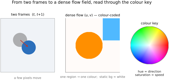
Optical flow is the two-dimensional motion vector of every pixel between two frames (usually consecutive): a dense field $\big(u(x,y),\,v(x,y)\big)$ that, for each pixel, says how far it moved horizontally and vertically. Because a field of little arrows is hard to read, flow is conventionally displayed with a color key: hue encodes the direction of motion and saturation its speed, so that a coherent moving region shows up as a smooth wash of one color (Figure 12.8.1).
This primitive earns its own chapter because almost everything downstream needs it. Frame interpolation and slow-motion synthesis transport pixels to the in-between time along the flow; video stabilization and compression both reduce to "estimate motion, then act on it"; super-resolution and inpainting align frames by it; and far outside photography, the same field drives optical mice, medical image registration, action recognition, egomotion and simultaneous localization and mapping (SLAM), and fluid-flow measurement. It is widely used.
A close relative shows what extra structure buys you. Stereo disparity is optical flow specialized to a static scene viewed by two cameras with a known baseline: the geometry forces the match to lie on a one-dimensional epipolar line, so there is a single unknown (depth, equivalently disparity) per pixel instead of two. Flow is the unconstrained two-dimensional version, with no epipolar line to ride and both components free (cross-ref Chapter 12.1, Brute force).
Brightness-based correspondence is ambiguous or invalid in several common situations:
- in flat, untextured regions there is simply no information, because nothing distinguishes one bit of blank sky from the next;
- at occlusion and motion boundaries, a pixel may have no correspondence at all because the thing it was looking at went behind something, or emerged from behind it;
- under lighting changes and specularities, brightness isn't constant, so the assumption everything below rests on quietly fails.
"The flow," then, is an idealization, and the math will warn us, pixel by pixel, where the idealization breaks. Keep that in mind: a flow field is a best effort, confident in some places and guessing in others, and good methods know the difference.
12.8.2 Brightness constancy and the optical-flow constraint⧉
Start from the one thing we are willing to assume is conserved as a point moves: its brightness. A scene point that sits at $(x,y)$ in the first frame and has slid by $(u,v)$ one timestep later should have the same intensity in the new location. It merely relocated, it did not change color:
Here $(u,v)$ is exactly the per-pixel displacement we are after. This is the brightness-constancy (or "color-constancy") assumption of Horn and Schunck (1981). It is an assumption, and we have already flagged where it breaks, for example a surface that turns toward the light, a specular highlight that slides across glass, or a pixel that gets occluded, but for small motions between consecutive frames it is serviceable.
As written, the equation is awkward: the unknowns $(u,v)$ sit inside the image function $I$, in a nonlinear way. The standard move is to linearize: expand the right-hand side to first order about $(x,y,t)$, assuming the motion is small:
where $I_x,I_y$ are the spatial image gradients and $I_t$ is the temporal gradient, in practice just the frame-to-frame difference at that pixel. Substitute this back into brightness constancy and cancel $I(x,y,t)$ from both sides, and the whole problem collapses to one clean line, the optical-flow constraint equation (OFCE):
Read it back: the flow, dotted into the image gradient, must cancel the temporal change. Two facts about this equation drive the entire rest of the chapter.
First, only the gradient carries motion information. Where the image is flat ($\nabla I = 0$), the constraint degenerates to $I_t = 0$ and says nothing whatsoever about $(u,v)$. You cannot see motion in a blank region, because nothing in it changes when it moves. All the information about flow lives in the image gradient, which is exactly why textureless regions were on our ill-posed list. (It is also the precise lever that Eulerian video magnification pulls from the other side: it amplifies the temporal change $I_t$ in proportion to the spatial gradient; cross-ref the motion-magnification chapter and Wu et al. 2012.)
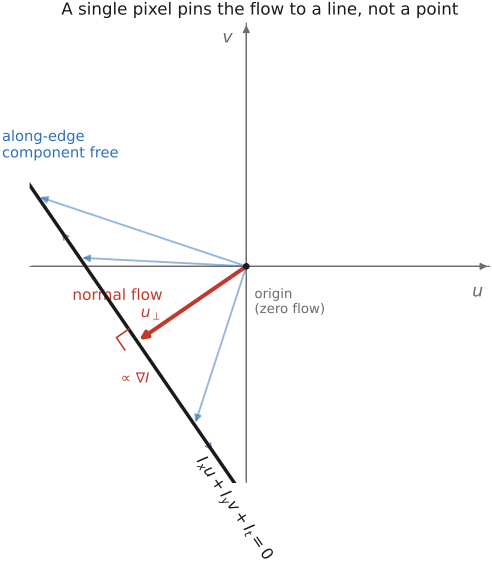
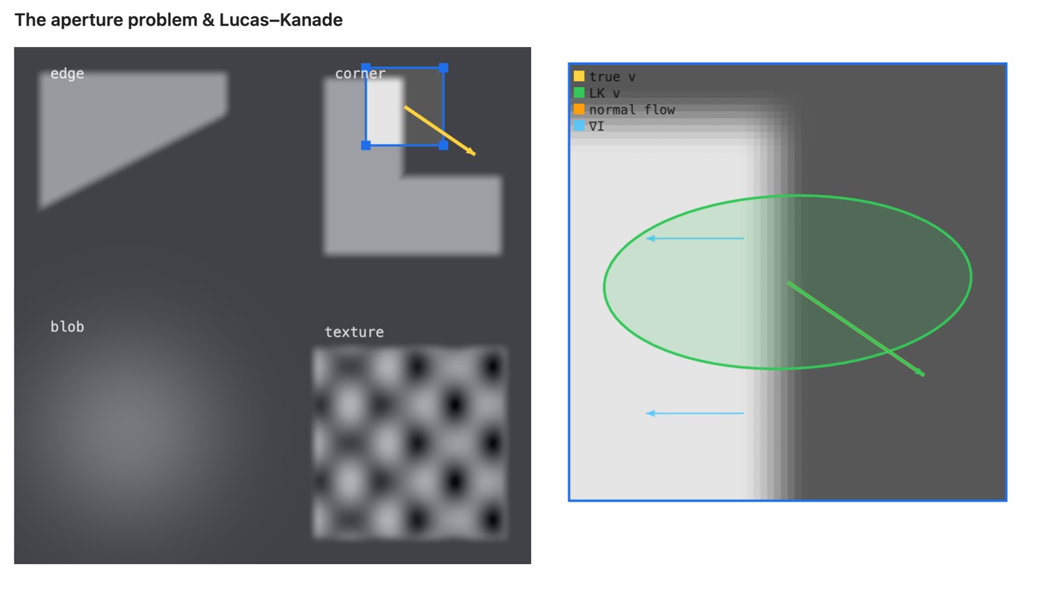
Second, this is the key point: one equation cannot determine two unknowns. The OFCE is a single scalar equation in the two unknowns $(u,v)$. In the plane of all possible flows it does not pick out a point; it picks out a whole line (Figure 12.8.2). The true flow lies somewhere on that line, but the single pixel cannot say where. The one thing we can read off is the component of motion along the gradient: the normal flow, of magnitude $u_\perp = -I_t / \lVert\nabla I\rVert$ directed along $\nabla I$. The component tangent to the edge is completely free. That under-determination has a name.
12.8.3 The aperture problem⧉
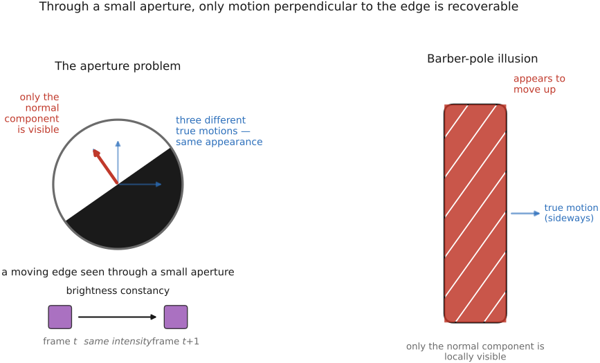
The under-determination we just met has a classical name and a vivid intuition: the aperture problem. The statement is exactly what the OFCE told us: from a single pixel you can recover only the normal flow, the motion perpendicular to the local edge; the motion along the edge is unobservable. One equation, two unknowns (Figure 12.8.3).
The intuition is the "aperture" the name refers to. Watch a long straight edge, a diagonal bar, slide behind a small round hole. You cannot tell whether the bar is moving horizontally, vertically, or straight perpendicular to itself: every one of those motions produces the same changing picture inside the hole. Only the component that changes what is visible through the aperture, the perpendicular one, registers; everything along the edge slides invisibly. The barber-pole illusion is the same effect in a perceptual setting: the diagonal stripes are physically rotating sideways around the pole, but because each stripe is a long edge, only the perpendicular (upward) component is locally visible, and the stripes appear to march up the pole forever.
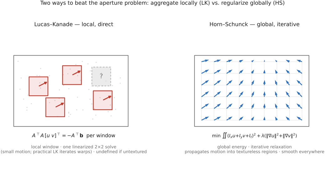
This is not a bug. The mathematics is reporting a real ambiguity in the data: a single local measurement does not determine tangential motion. So "solving" optical flow does not mean finding a cleverer way to invert one equation; it means adding a second assumption to supply the missing equation. The two classic choices, which organize the rest of the chapter, are:
- a local assumption, neighboring pixels share the same motion, which gives Lucas–Kanade;
- a global assumption, the flow field is smooth, which gives Horn–Schunck.
There is a perceptual coda. Human vision suffers the aperture problem too; we misperceive the barber pole and similar stimuli exactly as the equations predict, and the brain resolves it the same way the algorithms do: by integrating across the object, leaning on corners and line-endings (where there is no aperture ambiguity) to disambiguate the long edges. The math and the visual system are answering the same question with the same trick.
12.8.4 Lucas–Kanade: local constant-flow least squares (and the structure tensor)⧉
The first cure is local, and simple. Assume that all the pixels in a small window $W$ share the same motion $(u,v)$. That single assumption changes everything about the bookkeeping: instead of one equation in two unknowns, we now have many equations, one OFCE per pixel in the window, for the same two unknowns. The problem flips from under-determined to over-determined, and over-determined linear systems have a standard, robust answer: least squares. Aggregating the window both resolves the aperture problem (different pixels in a textured patch have differently-oriented gradients, so their constraint lines intersect at a point) and regularizes against noise. This is Lucas and Kanade (1981).
Concretely, stack the $n$ pixels of the window. Each contributes one row $[\,I_x \;\; I_y\,]$ and one entry $I_t$:
This is a tall, skinny over-determined system, and its least-squares solution is given by the normal equations, exactly the object from Chapter 6.7, Image formation as a linear system:
Solve the small least-squares system only where it has adequate rank and scale; do not explicitly invert a nearly singular matrix. But the real point is to look hard at that $2\times2$ matrix on the left, because we have met it before.
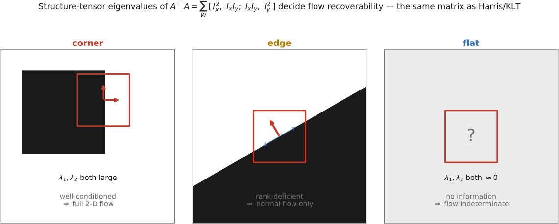
The matrix $A^\top A = \sum_W \left(\begin{smallmatrix} I_x^2 & I_x I_y \\ I_x I_y & I_y^2 \end{smallmatrix}\right)$ is the Harris structure tensor: the second-moment matrix of image gradients over the window, the very object that decided corner detection back in Chapter 12.3, Sparse matching (and originally Harris & Stephens 1988). The same matrix that found good keypoints now governs whether flow is recoverable, and its eigenvalues tell the whole story (Figure 12.8.4):
- two large eigenvalues: a corner or richly textured patch. $A^\top A$ is well-conditioned and invertible, so the full two-dimensional flow comes out cleanly. These are precisely Shi and Tomasi's "good features to track" (Shi & Tomasi 1994).
- one large eigenvalue: an edge. The matrix is rank-deficient; we recover only the normal flow, and the along-edge direction is its null space. This is the aperture problem, re-derived as a linear-algebra fact: the ambiguity is literally the unobservable eigenvector.
- both small: a flat region. No gradient information at all; the flow is indeterminate.
The unification is exact: the corner/edge/flat trichotomy that told us where to put keypoints for matching is the identical eigenvalue story that tells us where flow is well-posed because it is the same matrix. And it hands us the bridge to the next chapter: to get reliable sparse motion, just run Lucas–Kanade only on the pixels where $A^\top A$ is well-conditioned. That is exactly Kanade–Lucas–Tomasi (KLT) feature tracking (cross-ref Chapter 12.4, Feature tracking).
Two caveats fix Lucas–Kanade's scope. Because it rests on the same first-order linearization, it assumes small motion (on the order of a pixel); large displacements need the coarse-to-fine machinery below. Lucas–Kanade uses a shared displacement within a window, whereas Horn–Schunck estimates a globally coupled field; the local solve is not one iteration of that global model (Figure 12.8.6). The same gradient least-squares is also the engine of parametric image alignment (registering two whole images under one affine or projective warp), which is why Lucas–Kanade reappears in Chapter 12.1, Brute force: there the unknowns are a handful of warp parameters rather than a per-pixel $(u,v)$, but the normal-equations skeleton is the same.
12.8.5 Horn–Schunck: global smoothness regularization⧉
The second cure is global, and it supplies the missing equation from a prior rather than from a window. Instead of assuming constancy inside a patch, assume that the flow field as a whole is smooth, so neighboring pixels move similarly. This does something Lucas–Kanade cannot: it propagates motion from the data-rich places (corners, textured patches) into the data-poor ones (edges, flat regions), filling in the aperture-ambiguous directions from confident neighbors. This is the other half of Horn and Schunck (1981).
The assumption is expressed as an energy to minimize over the whole image, and it has the standard data-fit-plus-prior shape of every inverse problem in this book:
The data term is just the squared OFCE residual: it penalizes flow that violates brightness constancy. The smoothness term penalizes spatial variation of the flow, $\lVert\nabla u\rVert^2 + \lVert\nabla v\rVert^2$, i.e. it wants neighboring flow vectors to agree. The scalar $\lambda$ trades the two off: large $\lambda$ buys a smoother, more diffused field that fills the apertures aggressively; small $\lambda$ trusts the data and tolerates a noisier field.
Because the energy is quadratic in $(u,v)$, minimizing it is tractable in the most familiar way: the Euler–Lagrange equations are linear, a large sparse system that couples all the pixels (a screened-Poisson-like diffusion: the same flavor of system we solved in Chapter 6.7, Image formation as a linear system and again for Poisson editing). One does not form that matrix; one iterates (Gauss–Seidel or Jacobi), and each update has a readable form: every pixel's flow relaxes toward its neighborhood average, corrected by the local brightness constraint. Smooth the field, honor the data, repeat; the smoothness quietly carries motion into the textureless gaps where the data fell silent.
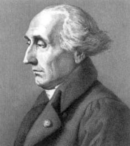 Joseph-Louis Lagrange (1736–1813) recast mechanics into the pure-calculus form we still use, and gave us the Euler–Lagrange equations, the recipe for the function that minimizes an energy. That is exactly what we just invoked to turn the Horn–Schunck smoothness energy (and, earlier, the Poisson blend) into a linear system to relax. His multipliers are the standard way to optimize under a constraint, and the Lagrangian "follow the particle" view of motion names the other half of the Lagrangian/Eulerian split of Chapter 12.4, Feature tracking. Napoleon made him a count; he chaired the commission that built the metric system. Portrait: public domain (via Wikimedia Commons).
The contrast with Lucas–Kanade is the thing to carry away (Figure 12.8.6): local window + least squares versus global field + smoothness prior; a one-step $2\times2$ solve versus an iterative sparse relaxation; constant-in-a-patch versus smoothly-varying-everywhere. They are two answers to the same question the aperture problem posed: supply the missing equation by aggregating locally or by regularizing globally.
A word on what "classical flow" actually means today, because the textbook Horn–Schunck is not what wins benchmarks. The Secrets of Optical Flow analysis of Sun, Roth and Black (2010) dissected the best classical methods and found the basic structure is still Horn–Schunck, but the improvements come from better terms: robust (non-quadratic, $L_1$/Charbonnier) penalties on both data and smoothness so that occlusions and motion edges do not get over-smoothed, median filtering of the flow between iterations, coarse-to-fine pyramids (next section), and edge-aware smoothness that bends the prior around image boundaries. The recurring lesson is that the choice of energy matters. Keep the data-fit-plus-prior scaffold and invest in penalties that match reality.
12.8.6 Large motion: coarse-to-fine warping⧉
Everything so far rode on the first-order Taylor expansion, and that expansion is only valid for sub-pixel motion. Real motion is many pixels. A hand can cross a quarter of the frame between two frames, and at that scale the linearization is simply wrong: the gradient at a pixel tells you nothing about a match twenty pixels away, and the solver either diverges or locks onto the wrong, aliased match. We need a way to make every motion look sub-pixel.
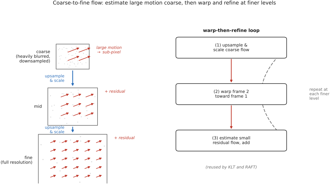
The fix is pyramids, and it reuses Chapter 6.6, Pyramids and wavelets wholesale. Build a Gaussian pyramid of both frames. On the coarsest level (heavily blurred and downsampled), a motion of, say, sixteen pixels in the original becomes a single pixel, which the linear method handles fine. Then walk back down toward full resolution, and at each finer level (Figure 12.8.7):
- upsample the coarse flow estimate to this level and scale its magnitude (twice the resolution → twice the displacement in pixels);
- warp frame 2 toward frame 1 by the current flow estimate, using the inverse-warp-and-resample engine of Chapter 11.1, Warping;
- estimate only the residual flow on the now-nearly-aligned pair (which is small again, so the linearization is valid) and add it to the running estimate.
Repeat to the finest level. The warp-then-refine loop is worth memorizing, because it is precisely the iterative scheme the learned methods at the end of the chapter reproduce, except that the per-step update is learned rather than derived:
flow = zero field on the coarsest grid
for each level from coarsest to finest:
    if this is not the coarsest level:
        resize flow and scale x/y components by their coordinate-scale ratios
    repeat up to an iteration cap:
        r(x) = frame2(x + flow(x)) - frame1(x)
        J(x) = gradient(frame2) sampled at x + flow(x)
        solve the chosen weighted/regularized linearized problem for delta
        reject invalid updates; flow = flow + delta
        stop if the declared step and residual criteria are met
return flow and validity/confidence information
A pyramid increases the range of motions accessible to a local linearization. It is not a Laplacian decomposition of the true motion, and downsampling can erase small moving objects. Iterative refinement cannot recover evidence that was lost at coarse levels without additional matching or a better initialization.
A different attack on large motion abandons the linearization entirely and matches patches directly. For each pixel in frame 1, score its similarity (sum-of-squared-differences, or correlation) against every candidate offset in frame 2; the result is a cost volume: a high-dimensional table of match scores over all displacements. This keeps brightness constancy but drops the Taylor approximation, so it handles arbitrarily large motion at the price of an expensive search (pruned in practice by coarse-to-fine and, soon, by learned features). The cost volume is a sideshow in classical flow but the centerpiece of the learned methods we turn to now.
For the fixed linearized Horn–Schunck energy above, the stationarity equations are
Use a smoothness discretization and boundary conditions consistent with this energy. In completely uninformative regions, smoothness extrapolates motion rather than measuring it; constant-flow null modes can remain if the data supplies no anchor. Evaluate endpoint error on known visible motion separately from occlusion handling. Forward/backward consistency must sample the backward field at the displaced coordinate, not compare the two fields at the same pixel.
12.8.7 Learned flow: RAFT (neuralize the classical pipeline)⧉
Learned methods can replace the representation and update rule. RAFT is a useful architectural example Teed & Deng 2020, not a permanent statement about which model leads every benchmark.
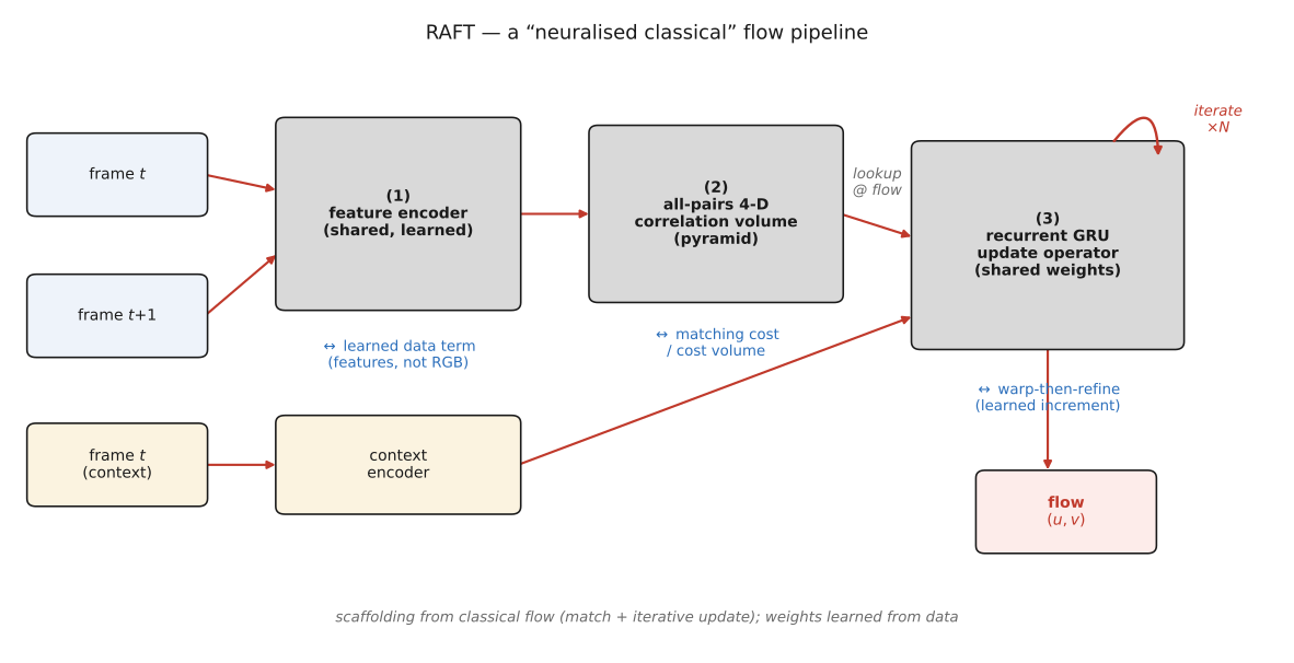
The exemplar is RAFT (Teed and Deng 2020, a European Conference on Computer Vision (ECCV) best paper), and it is best read as the classical pipeline with three of its parts neuralized (Figure 12.8.8):
- learned per-pixel features replace raw RGB in the matching, so a match survives lighting changes and weak texture that would break brightness constancy on pixels, plus a separate context encoder of frame 1 that supplies the edge-aware regularization Horn–Schunck got from a smoothness prior;
- an all-pairs 4-D correlation (cost) volume: the cost volume from the previous section, computed between every pair of locations on the lower-resolution feature grids and pooled into a pyramid for cheap multi-scale lookup;
- a recurrent update operator (a GRU with shared weights) that iteratively refines the flow: at each step it looks up correlations at the current flow estimate and predicts an increment, which mimics an iterative optimizer, the unrolled cousin of the warp-then-refine loop from the last section, but with the update learned instead of derived.
The whole thing is differentiable and trained end-to-end. Two notes earn their place. First, flow got the deep-learning treatment relatively late because it is intrinsically non-local: a pixel can match anywhere in the other frame, which ordinary convolutions, with their small receptive fields, handle badly. The explicit cost volume is the inductive bias that makes non-local matching tractable, and it is no accident that RAFT keeps it. Second, ground-truth flow is hard to obtain for real scenes, so training leans on synthetic datasets such as FlyingChairs, FlyingThings3D Mayer et al. 2016 (FlyingThings3D) and Sintel Butler et al. 2012 (Sintel), real driving data such as KITTI Geiger, Lenz & Urtasun 2012 (KITTI) and on self-supervised warping losses that score a flow by how well it warps one frame onto the other.
Synthetic large-motion flow benchmark; real driving flow with sparse GT. <http://sintel.is.tue.mpg.de> · <https://www.cvlibs.net/datasets/kitti/>. See the Chapter 45.16, Datasets appendix.
This is exactly the part's lesson about learned methods: RAFT is the classical pipeline with its hand-crafted parts replaced by learned ones. The structure comes from the classical method, and the operators are learned from data. It is pointedly not a generic transformer that dissolved the structure into attention: its cost volume and recurrent update show how problem-specific structure can help a learned model solve non-local matching (the lineage runs FlowNet 2015 Dosovitskiy et al. 2015, the first convolutional neural network (CNN) flow → PWC-Net 2018 Sun et al. 2018, an explicitly pyramid + warping + cost-volume, "Lucas–Kanade-flavored" net → RAFT and its transformer variants).
And with a dense, automatic correspondence field finally in hand, the transport half of the part opens up: warp and interpolate between frames for slow-motion synthesis, stabilize, compress with motion-compensated prediction, magnify subtle motion, or lift the field to its three-dimensional cousins (scene flow, structure-from-motion). Correspondence first, then transport: the flow we just estimated is the correspondence, and the rest of this part spends it.
Recap: big lessons of this chapter
Correspondence first, then transport. The unifying move of this whole part: nearly every technique (1) estimates a correspondence (a coordinate map saying where each pixel came from) and then (2) transports the pixels along it by warping and resampling. The transport is one shared engine (Chapter 11.1, Warping); the correspondence is the hard, ill-posed part. Optical flow is the part's most general correspondence estimator: a dense, per-pixel map estimated automatically from two images, where a homography would be parametric and a morph field user-drawn. Here, the flow is the correspondence: the field $(u,v)$ is itself the coordinate map that morphing, frame interpolation, stabilization, and compression all transport along. Everything downstream of this chapter assumes you can produce it. This is the part's anchor for L17 (registered in Matching pixels across space and time; it recurs across the part).