12.3 Sparse matching🔗⧉

The previous part transported pixels along maps that were given or hand-drawn. This part estimates the maps, and the cheapest, most robust way to start is not to match every pixel but to match a sparse handful of points you can find again. The pipeline has three stages, in order: detect distinctive points, describe each neighborhood with a vector, then match those vectors across images. Two design goals govern the whole pipeline and pull in opposite directions. Detection must be repeatable: the same physical point should fire in both images despite a change of viewpoint, zoom, and lighting. If a corner is found in one image but not the other, there is no chance to match it. Description must be distinctive yet invariant: unique enough that the right match stands out unambiguously, but stable enough to survive the change between the two images. Repeatability and distinctiveness are the two halves of the contract, and almost every design decision below is a negotiation between them.

12.3.1 Where to look: corners, and the structure tensor🔗⧉

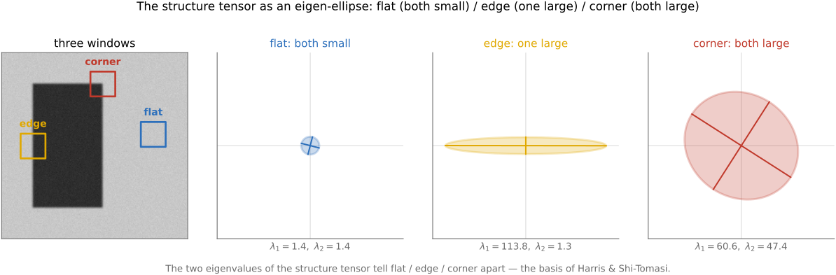
Why corners? Because a point can only be localized where the intensity changes in both directions. Walk through the three cases (Figure 12.3.1⛶ fullscreen). A flat patch can be slid in any direction and looks identical, so there is nothing to lock onto, and its position is hopeless. An edge is worse than it looks: you can slide it along itself and see no change, so its position along the edge is unrecoverable. This is the aperture problem of Chapter 12.8, Optical flow, now seen in detection. Only a corner, where two differently oriented edges meet, pins down uniquely, because every small shift changes the appearance.

The quantitative test for "varies in both directions" is the structure tensor $M$, also called the second-moment matrix or, in this context, the Harris matrix. Imagine shifting a window $W$ by a small $(\Delta x,\Delta y)$ and measuring the resulting sum-of-squared-differences; a first-order Taylor expansion turns that error surface into a quadratic form whose matrix is exactly

the gradient outer products $\nabla I\,\nabla I^{\top}$ accumulated over the window with weights $w$ (a Gaussian, in practice, for a smooth falloff). The two eigenvalues $\lambda_1\ge\lambda_2$ of $M$ measure how strongly the intensity varies along its two principal directions, and they read off the three cases cleanly: flat means both eigenvalues tiny ($M$ near zero, the error surface nearly flat); edge means one large eigenvalue and one near zero ($M$ rank-deficient, the error surface a trough); corner means both eigenvalues large ($M$ well-conditioned, the error surface a steep bowl). Drawn as an error ellipse with axes $\lambda_1^{-1/2},\lambda_2^{-1/2}$, the partition is one picture: an unbounded tangent direction for an ideal edge, little constraint in either direction for a flat patch, and bounded uncertainty in both directions for a sufficiently informative corner.

Two responses turn the eigenvalues into a detector. Harris (Harris & Stephens 1988 Harris & Stephens 1988) avoids computing eigenvalues, which were expensive in 1988, and uses the cheap determinant-and-trace combination

with $k\approx 0.04$–$0.06$. $R$ is large and positive only when both eigenvalues are large (a corner), strongly negative on edges (one eigenvalue dominates), and near zero on flat regions. The pipeline is then mechanical: compute gradients, form the three products $I_x^2, I_y^2, I_xI_y$, Gaussian-smooth each, combine into $R$, threshold, and non-maximum-suppress so each corner fires exactly once (Figure 12.3.2⛶ fullscreen). A useful property falls out for free: because $R$ is built from gradients it is invariant to an intensity offset ($I\to I+b$), and because the structure-tensor ellipse merely rotates with the image, $R$ is invariant to image rotation; only the absolute scaling of the threshold and, as we will see, the image scale give it trouble.

Shi–Tomasi (Shi & Tomasi 1994 Shi & Tomasi 1994, "good features to track") takes the more direct route and scores a corner by the smaller eigenvalue itself,

a point is a good corner exactly when its weaker direction is still strong, i.e. both directions are well-constrained. This is the same criterion that makes a feature trackable (it is precisely the condition that $M$ be well-conditioned for the KLT motion solve in Chapter 12.4, Feature tracking), which is why Shi & Tomasi derived "what is a good feature to detect" from "what is a good feature to track." Harris versus Shi–Tomasi is two readings of the same matrix: Shi–Tomasi is slightly more reliable, Harris slightly cheaper, and in practice they pick nearly the same points.

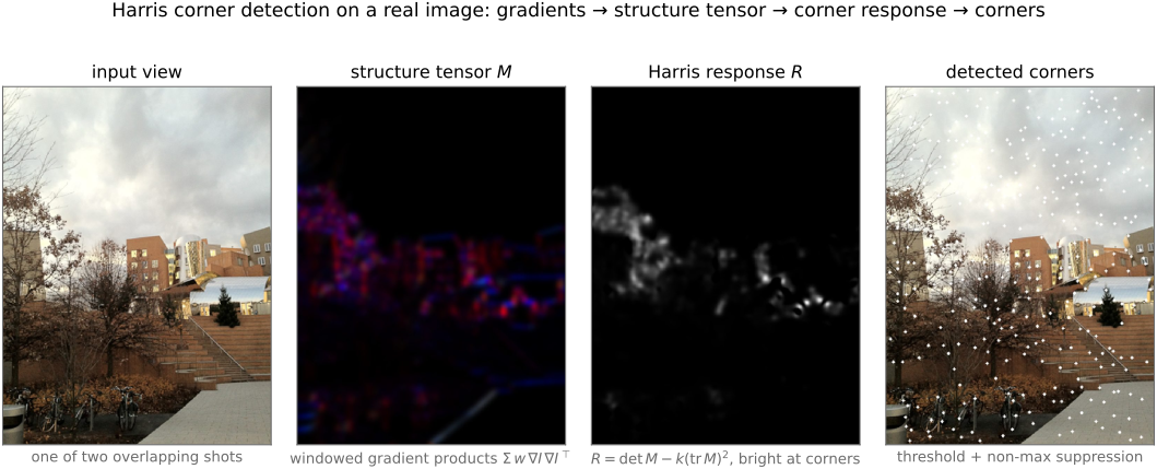
Apply nonmaximum suppression after a corner response and retain spatial coverage, not only the strongest cluster. Thresholds depend on image scale, derivative filters, encoding and noise. Large tensor eigenvalues describe local translation sensitivity; they do not guarantee a correct correspondence across viewpoints.

12.3.2 Invariance: surviving scale and rotation🔗⧉

Harris solves where to look within a single image, but a corner detected at one zoom or one orientation must be found, and described the same way, in an image where the object is bigger or rotated. Across far views this is the crux: the two photos differ in scale (you stood closer, or zoomed) and in rotation (you tilted the camera, or the object turned). Plain Harris fails the scale test outright. Blur an image down and a corner becomes a smooth bump that the detector reads as flat, or as an edge. Repeatability across far views therefore demands that detector and descriptor be covariant with scale and rotation: find the same physical point, and measure its neighborhood in a frame that rotates and scales with the point itself.

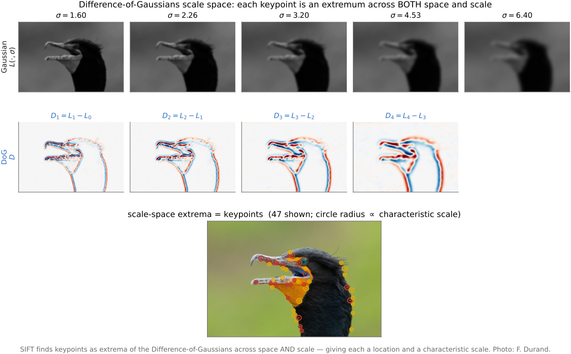
Scale is SIFT's signature contribution (Lowe 2004 Lowe 2004). The idea is to give each keypoint its own characteristic scale, found automatically and consistently across images. Build a scale-space, the image repeatedly blurred by a Gaussian of growing $\sigma$, so that fine structure dissolves as you climb, and look for a function of $\sigma$ that peaks at the size of the structure under the point. A center-surround / band-pass response does exactly this: it is near zero when the window is much smaller or much larger than the feature and peaks when they match. SIFT computes it cheaply as the Difference-of-Gaussians,

a close and inexpensive approximation to the scale-normalized Laplacian. A keypoint is then a point that is a local extremum of $D$ in all three coordinates jointly, a maximum or minimum over $(x,y)$ and over neighboring scales $\sigma$ (Figure 12.3.3⛶ fullscreen). The scale at which the extremum occurs is the feature's characteristic scale: describe the neighborhood at that scale, and the descriptor no longer cares how zoomed-in the photo was. (In practice the scale-space is organized into octaves, halving the resolution each octave, and the raw extrema are refined to sub-pixel, sub-scale precision by fitting a quadratic, with weak or edge-like extrema discarded by a DoG-value threshold and a principal-curvature ratio test, the Harris idea reused to reject points strung out along an edge.)

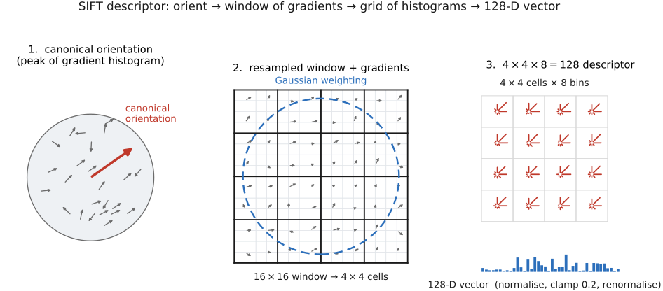
Rotation is handled by an analogous canonical-frame trick. Around the keypoint, at its scale, build a histogram of local gradient orientations (weighted by gradient magnitude) and read off its peak: the dominant orientation. Then measure the descriptor relative to that orientation, as if the patch had been rotated to a canonical upright pose. Rotate the object in the world and its dominant orientation rotates with it, so the descriptor comes out unchanged. Illumination invariance is bought the same cheap way it was for Harris: use gradients, which are blind to an additive brightness offset, and normalize the final vector to remove a multiplicative gain. With characteristic scale and dominant orientation in hand, every keypoint comes with a stable local coordinate frame $(x,y,\sigma,\theta)$, and the descriptor's only remaining job is to summarize what the neighborhood looks like in that frame.

12.3.3 Describing a neighborhood: SIFT and its zoo🔗⧉

The simplest possible descriptor is the raw patch, a small window of pixel values around the keypoint, matched by SSD or NCC. It is invariant to nothing on its own; bolted onto the canonical frame above (resample the window at the keypoint's scale, rotate it to the dominant orientation, normalize its intensities) it becomes serviceable, and this is essentially the Multiscale Oriented Patches descriptor. But raw patches are brittle: a one-pixel misregistration or a small non-rigid deformation changes every value, so the SSD jumps. The standard improvement is to describe the patch by its gradients, histogrammed over cells, which makes it distinctive yet tolerant of those small shifts.

That is SIFT (Lowe 2004 Lowe 2004), the Scale-Invariant Feature Transform, and here it is concretely (Figure 12.3.4⛶ fullscreen). Take a $16\times16$ window around the keypoint, sampled at the feature's scale and rotated to its dominant orientation. Divide it into a $4\times4$ grid of cells. In each cell, accumulate the gradient orientations into an 8-bin histogram, each gradient weighted by its magnitude and by a Gaussian centered on the keypoint (so the window edges count less), and spread across bins by trilinear interpolation (so a gradient near a cell or bin boundary does not flip discontinuously). Concatenate the $4\times4$ cells $\times\,8$ orientations into a single 128-dimensional vector. Finally, $L_2$-normalize it, then clamp every component to a ceiling (0.2) and renormalize, which blunts the influence of a few very large gradients from, say, a strong specular edge. The important design choice is the histogram: by binning gradients within a cell rather than recording their exact positions, SIFT tolerates small spatial shifts and deformations while remaining highly distinctive, the resolved tension between invariance and discriminability. Empirically it survives viewpoint changes up to roughly $60^\circ$ of out-of-plane rotation and dramatic illumination shifts, which is why it dominated matching, stitching, and recognition for a decade.

SIFT is accurate but not cheap, and a zoo of successors trades accuracy for speed along a single set of trade-offs: speed, robustness, and invariance (Figure 12.3.5⛶ fullscreen). SURF (Bay et al. 2006) Bay et al. 2006 (SURF) approximates SIFT's Gaussian derivatives with box filters evaluated in $O(1)$ via the integral image, buying a large speed-up for a small robustness cost. FAST (Rosten & Drummond 2006) Rosten & Drummond 2006 (FAST) is only a corner detector; it tests pixels on a circle for a contiguous arc brighter or darker than the center, extremely fast, with no descriptor of its own. The binary descriptors are the real-time workhorses: BRIEF (Calonder et al. 2010) Calonder et al. 2010 (BRIEF) encodes a patch as a string of bits, each one the answer to "is pixel $p$ brighter than pixel $q$?" for a fixed set of test pairs, and ORB (Rublee et al. 2011) Rublee et al. 2011 (ORB) wraps FAST detection plus a rotation-aware BRIEF into a complete, patent-free, SIFT-free pipeline; BRISK Leutenegger, Chli & Siegwart 2011 (BRISK) adds a scale-space and a structured sampling pattern. Binary descriptors are tiny and are matched not by Euclidean distance but by Hamming distance: a XOR and a popcount, almost free on modern hardware. At the other end, KAZE Alcantarilla, Bartoli & Davison 2012 (KAZE) / AKAZE Alcantarilla, Nuevo & Bartoli 2013 (AKAZE) build their scale-space with nonlinear (edge-preserving) diffusion instead of Gaussian blur, respecting object boundaries for better localization at higher cost. In short, SIFT remains the accuracy benchmark; binary descriptors are what you reach for when you need thousands of matches per frame on a phone.

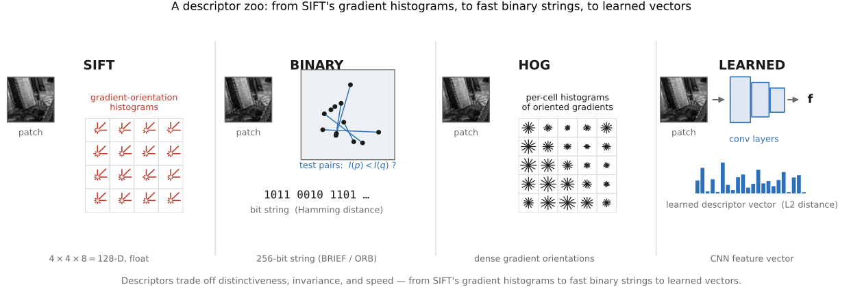
Canonical scale and orientation reduce sensitivity to those transformations but do not guarantee invariance under severe perspective change, blur or occlusion. For descriptors, use Euclidean distance for an appropriately normalized SIFT vector and Hamming distance for binary descriptors such as ORB. Compare performance under the image changes expected in the application.

12.3.4 Matching: nearest neighbor in descriptor space🔗⧉

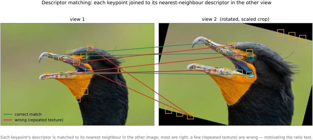
With every keypoint reduced to a vector, matching is conceptually trivial: a keypoint in image A matches the keypoint in image B whose descriptor is nearest (Figure 12.3.6⛶ fullscreen). The distance is Euclidean for float descriptors (SIFT, SURF) and Hamming for binary ones (ORB, BRIEF). Done naively, this is exhaustive: compare every descriptor in A against every descriptor in B, which is fine for a single pair of images but becomes the bottleneck once you match against a large database (Photo Tourism reconstructs cities from tens of thousands of photos, each with hundreds of features). The standard remedy is approximate nearest-neighbor search (k-d trees with best-bin-first, or modern hashing) which trades a small chance of missing the true nearest neighbor for an enormous speed-up; the details live in Chapter 12.7, Fast matching.

A caveat is that the raw nearest-neighbor matches are not ready to use. Repeated texture (a row of identical windows, a brick wall), occlusion, and ordinary descriptor collisions all manufacture matches that are confident but wrong, and a single wrong correspondence can wreck a least-squares fit of the transform you ultimately want. The fix is two-stage and is the subject of the next section: Lowe's ratio test prunes ambiguous matches before fitting (accept a match only if the nearest descriptor is decisively closer than the second nearest), and then RANSAC Fischler & Bolles 1981 fits a geometric transform robustly despite whatever outliers survive. That is Chapter 12.5, Robustness: the ratio test and RANSAC, which this section feeds, and from there the clean correspondences flow into panorama stitching (Chapter 20.2, Automatic panorama stitching from multiple views and feature matching) and 3-D reconstruction (Part 36, 3D and depth). The entire hand-designed pipeline, detector, descriptor, and matcher, is exactly the kind of three-stage system that later learned methods replace, swapping each stage for a learned operator (SuperPoint DeTone et al. 2018 (SuperPoint), SuperGlue Sarlin et al. 2020 (SuperGlue), and the pointmap regressors of Chapter 12.6, Deep learning approaches to sparse matching); but the problem it solves is the one stated here, and SIFT remains the baseline they are measured against.