12.1 Brute force⧉
Every multi-frame method you will meet in this book, including burst denoising, HDR merging, panorama stitching, focal stacking, and super-resolution, silently assumes that corresponding scene points already sit on the same pixel in every frame. They do not. Hand tremor jitters a hand-held burst; the sky rotates through a long-exposure astrophotograph; a tripod drifts; the subject breathes. Combining frames that disagree by even a pixel does not clean the image. It blurs it. So before any of those methods can run, the frames must be registered, and registration is the subject of this chapter.
We will pose it as a single optimization and then spend the rest of the chapter on how to solve it. The cleanest version takes the smallest possible transform, a pure 2-D translation, because it is simple, it is a problem-set algorithm, and it exposes every idea the richer families (a homography for a panorama, a dense field for flow) will reuse.
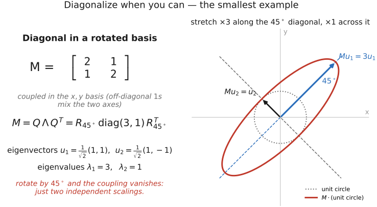
A pure translation is diagonal in the Fourier basis: it leaves every frequency magnitude untouched and tilts only the phases, by a ramp whose slope is the shift. So a brute-force $O(n\,\text{window}^2)$ shift search over $n$ samples collapses to a single FFT pair: form the normalized cross-power spectrum, inverse-transform, and read the shift off the location of the resulting spike. Whenever the operator you face is a shift, a convolution, or a correlation, ask first whether the frequency domain turns the work into a per-frequency (diagonal) operation. (L6.8 is first placed in Chapter 6.3, Fourier; here it turns a search into a transform.)
12.1.1 Why you must align first⧉
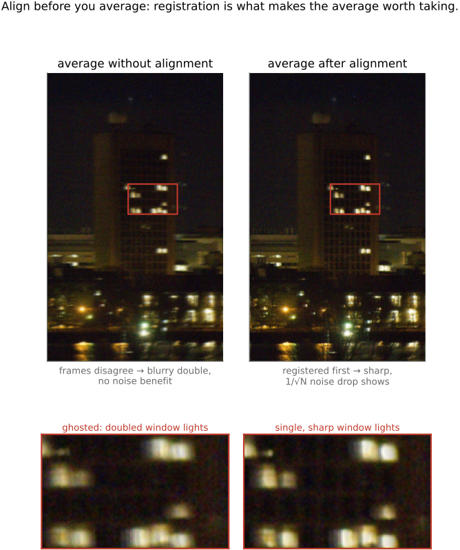
Recall the law behind burst photography: average $N$ independent frames of the same scene and the noise falls by $1/\sqrt N$ while the signal stays put. That law has a precondition: it only holds if the frames are registered, so that the same scene point contributes to the same output pixel in every frame. Average a hand-held burst without aligning it and you do not get the clean $1/\sqrt N$ image; you get a blurry double (Figure 12.1.1). Alignment is not optional. It is what makes the noise reduction possible in the first place.
It helps to name the two failure regimes, because they look different and cost differently. A sub-pixel misalignment blurs: the mean low-passes across the small offset, and you get one image, softer. A whole-pixel-or-more misalignment ghosts: every edge appears twice, the unmistakable signature of an unregistered stack. Deep-sky astrophotography is the extreme case. Over a long session the sky rotates through the field, so without per-sub-exposure alignment the stars trail and the whole stack mushes into smear rather than resolving faint detail.
Formally, alignment is an inverse problem: find the transform $T$ that makes the second frame, re-sampled through $T$, agree with the first,
Everything in this chapter is two choices made inside this objective: which family $T$ is drawn from (translation here; a homography for camera rotation and panoramas; a per-pixel field for flow, next), and how you search that family. This is exactly the correspondence-first half of the part's main idea (L17): recover the map $T$, and the downstream transport, the averaging, the merging, and the stitching, follows automatically.
12.1.2 Brute-force translational alignment (SSD / NCC)⧉
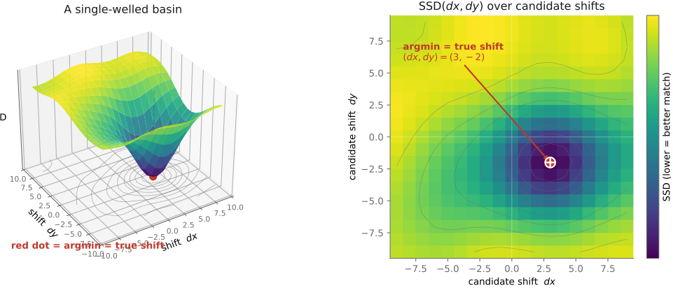
For a tight burst the whole image slides as one rigid 2-D shift $(dx,dy)$, and the simplest aligner imaginable just tries every shift in a search window and keeps the best-scoring one. A double loop over $(dx,dy)$, with no cleverness at all, is useful here because it leaves little room for implementation errors. Everything then rides on the score: the function that says how well two frames agree at a given candidate shift (Figure 12.1.2).
The default score is the sum of squared differences (SSD),
SSD is small when the sampled intensities agree, which need not happen at a unique displacement. Repeated patterns create several minima; flat regions create weak curvature. Same exposure does not guarantee brightness constancy, and an HDR bracket can add clipping and motion. Mean-subtracted normalized cross-correlation handles a positive affine intensity change on the evaluated region:
NCC subtracts the mean and divides by the norms of the centered patches. It is invariant to positive gain and constant offset when neither patch is constant. Mask clipping and invalid pixels; do not divide by nearly zero variance. Nonlinear tone changes and spatially varying illumination require a better model than a single gain and offset.
Two practical notes. First, the cheapest unit test you will ever write: align a synthetic image to a known shift of itself and confirm the minimum lands exactly there, by construction. Catch the indexing, sign, and interpolation bugs on that toy, not on noisy real frames where a one-pixel error hides in the grain. Second, sub-pixel accuracy: the integer-grid minimum is rarely the true minimum, so fit a parabola to the SSD basin (or upsample the surface) and read off the vertex to get a fractional shift, realized by bilinear or bicubic interpolation when you resample. Those tiny fractional offsets are noise to be removed when you are denoising, but they are signal to be exploited when you are super-resolving: a burst whose frames are sub-pixel-shifted samples the scene more densely than any one frame can, which is precisely what burst super-resolution mines (Wronski et al. 2019 Wronski et al. 2019; cross-ref Chapter 14.2, Multi-frame super-resolution).
Prokudin-Gorsky’s sequential color-separation captures provide an early alignment example Prokudin-Gorskii. NCC can be a useful baseline for their digitized channels, but spectral color differences are not generally a single gain and offset. Gradients, suitable crops and rejection of damaged or moving regions may improve the estimate (Figure 12.1.4).
Both steps can be run on a real burst: search the window, read off the shifts, and average with and without them (Figure 12.1.3).
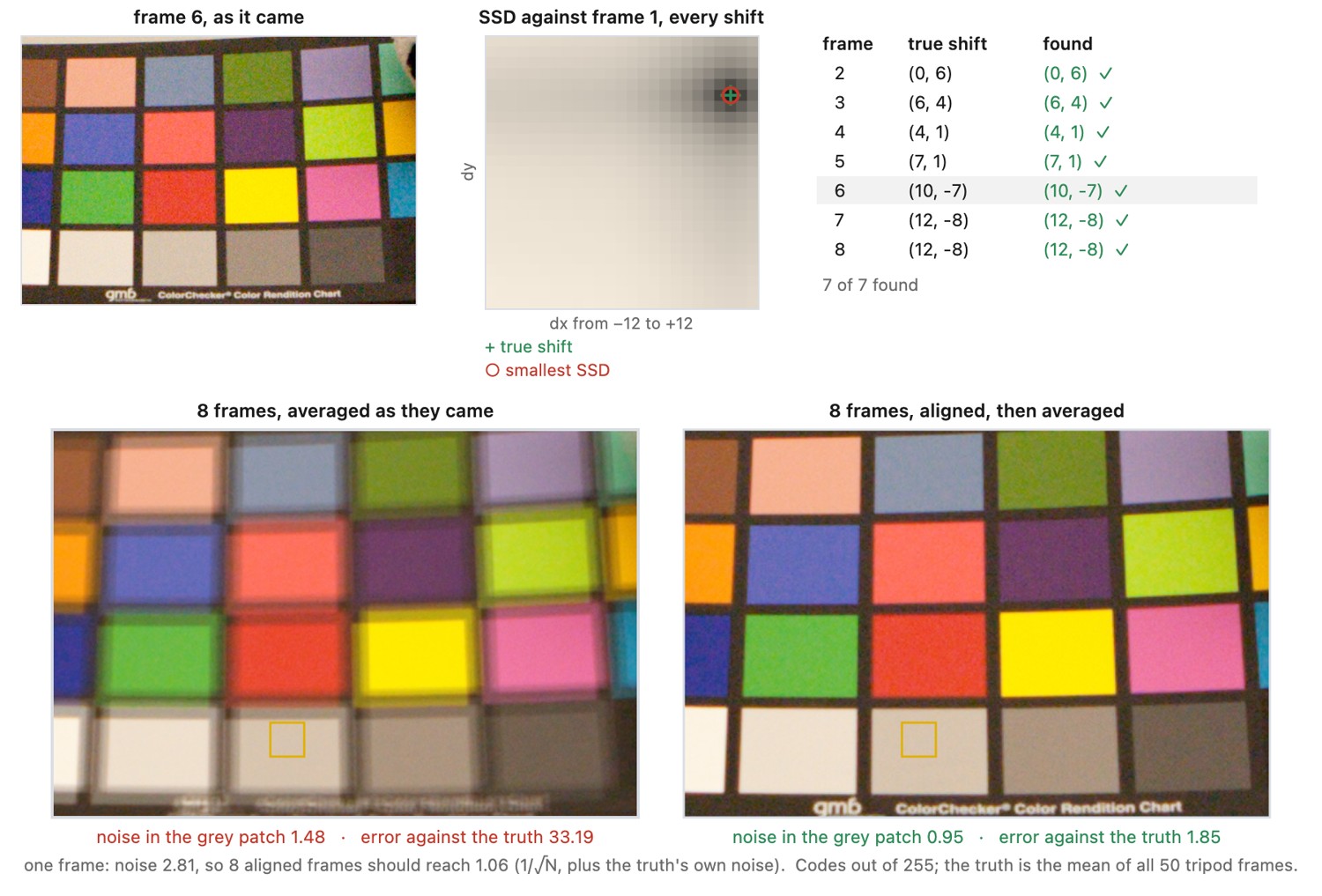
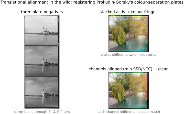
Compare candidate shifts over a common valid support, or normalize a masked score by a sufficient valid-sample count. Otherwise larger shifts can win merely by discarding difficult pixels. A low residual and a high margin over competing shifts are complementary checks; neither detects all model mismatch.
The separated color exposures of Prokudin-Gorsky provide a useful application Prokudin-Gorskii. Shifted channels turn an otherwise sharp edge into red and cyan fringes when the plates are stacked. Search for a translation of each channel relative to a reference and inspect whether those fringes shrink. However, a red object can be bright in one filtered exposure and dark in another. Normalized correlation compensates for a common offset and scale, not for every spectral difference between objects. Comparing gradients or selecting regions with shared structure can help. Motion between exposures remains a separate problem that a single channel translation cannot fix.
12.1.3 Phase correlation: the whole shift from one FFT⧉
Brute force is straightforward but wasteful: an $O(n\,\text{window}^2)$ direct search over $n$ compared samples to find a single shift. There is a way to read the shift off in one shot, and it comes straight from the shift theorem (L6.8, Chapter 6.3, Fourier). A pure translation multiplies the spectrum by a pure phase ramp and changes nothing else:
The entire translation lives in the phase, encoded as a ramp whose slope is the shift. The magnitudes are untouched, which is the diagonalization the big lesson promised.
Phase correlation (Kuglin & Hines 1975 Kuglin & Hines 1975) turns this observation into an algorithm. Form the normalized cross-power spectrum,
The overbar denotes complex conjugation. Under the stated convention $I_2(x)=I_1(x-d)$, this ordering gives $R=e^{+i\omega\cdot d}$, whose inverse transform peaks at $-d$. Negate that peak to obtain the forward displacement $d$, or reverse the conjugation order. The reason the answer is a spike rather than a broad bump: a delta at position $x_0$ has the spectrum $e^{-i\omega\cdot x_0}$, unit magnitude at every frequency and a linear phase. Normalizing the cross-power gives every frequency unit magnitude too, so $R$ is exactly the spectrum of a delta at $-d$. Seen in the image domain, every frequency's cosine reaches its crest at that one location and they cancel everywhere else. Verify this with a known synthetic shift. Suppress or regularize bins of negligible cross-power before normalization. DFT shifts are periodic; padding/windowing and overlap handling change practical behavior. Peak shape is useful evidence but not a calibrated probability of correctness.
Rotation and scale estimation can use log-polar resampling of Fourier magnitudes, where those transformations become shifts under the model. This is not equivalent to applying log-polar coordinates directly to two arbitrarily translated images. Sampling, finite support and symmetry still create ambiguities.
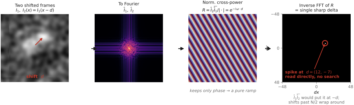
Normalizing the cross-power removes the magnitude factor from a positive global exposure gain, leaving the phase that locates the shift. A constant offset affects the DC term; clipping, spatially varying light and nonlinear encoding are different changes. The transform computation costs on the order of the number of pixels times its logarithm, and avoids evaluating a full image residual for every candidate shift. It still estimates one global translation. Parallax and independently moving subjects require local motion models or rejection, not a more confident reading of the same peak.
12.1.4 Coarse-to-fine alignment on a pyramid⧉
Brute force has two failure modes that bite together. Large motion forces a large, and therefore expensive, search window; and a raw SSD surface is not always the clean single-welled basin of the idealized figure. Repetitive texture (a brick wall, a picket fence) and aliasing carve local minima into it, and a local refinement started far from the answer can fall into the wrong well. An exhaustive search finds the best score in its window, though that score may favor a false match. Going multiscale addresses both, though only the first reliably (Figure 12.1.6).
Build a Gaussian pyramid of both frames and align coarse-to-fine (the pyramid of Chapter 6.6, Pyramids and wavelets, here repurposed as a search strategy). At the tiny, heavily-blurred top of the pyramid, a small search in pixels covers a large real motion, because each coarse pixel stands for many fine ones, so large displacements become cheap. Better still, the low-frequency surface at the top may be smoother because blurring attenuates high-frequency detail, often making a rough estimate easier to obtain. Propagate that estimate down to the next level, scale it up, and refine it with a tiny local search; the high frequencies you add as you descend mostly refine the estimate, because the local search at each level is too small to jump to a distant minimum. That is also the risk: if the coarse estimate is wrong, the finer levels rarely recover.
Pyramids can smooth the cost and reduce a large displacement to a smaller coarse-grid shift. They do not guarantee one clean basin: periodic texture and lost small structures can remain ambiguous. Verify the refined result on the original images.
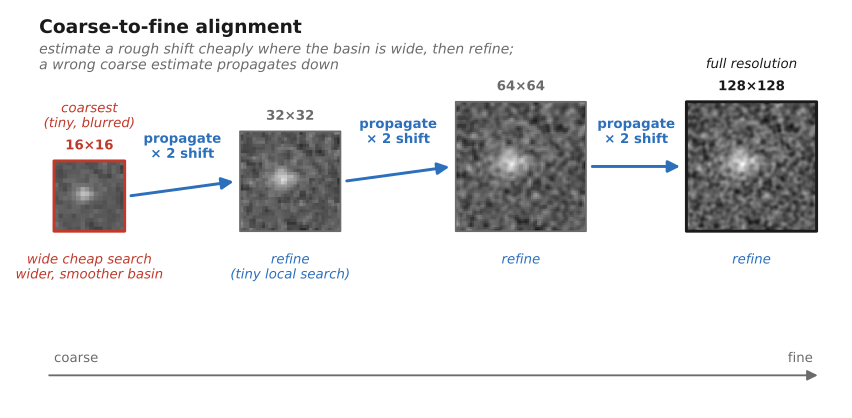
Build each level by filtering before decimation. Otherwise the coarse image can contain alias patterns that disagree between frames, creating false evidence for motion. A pyramid is useful both as a representation and as a search strategy: solve large motions on a coarse grid, then recover precision from finer samples. HDR+ applies this idea to tiles before robust burst merging Hasinoff et al. 2016. Local refinement should still be checked against alternatives when the coarse choice is ambiguous.
Recap: big lessons of this chapter
A pure translation is diagonal in the Fourier basis: it leaves every frequency magnitude untouched and tilts only the phases, by a ramp whose slope is the shift. So a brute-force $O(n\,\text{window}^2)$ shift search over $n$ samples collapses to a single FFT pair: form the normalized cross-power spectrum, inverse-transform, and read the shift off the location of the resulting spike. Whenever the operator you face is a shift, a convolution, or a correlation, ask first whether the frequency domain turns the work into a per-frequency (diagonal) operation. (L6.8 is first placed in Chapter 6.3, Fourier; here it turns a search into a transform.)