11.2 Antialiasing for complex transforms🔗⧉

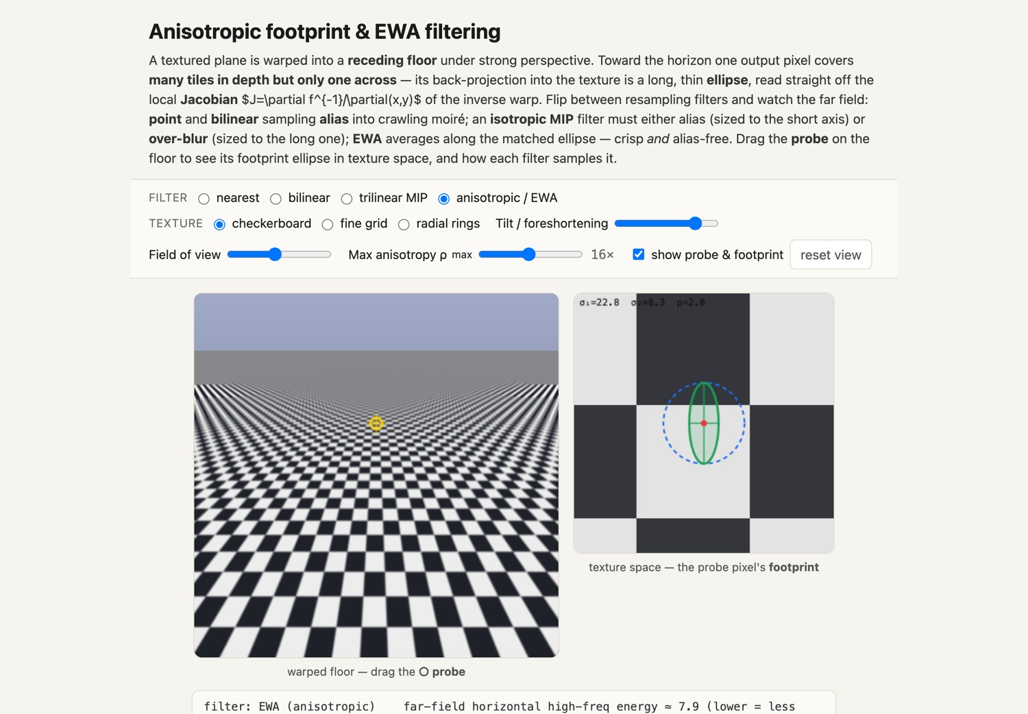
Take the warp engine of the previous chapter and point it at a checkerboard floor receding to the horizon. Near the camera, one output pixel covers about one tile, and the round prefilter of Chapter 11.1, Warping handles it perfectly. But follow the floor into the distance and something breaks: toward the horizon a single output pixel spans many tiles in depth while still covering only one tile across. The patch of source that lands in that pixel is not a little square. It is a long, thin sliver, dozens of times longer than it is wide. Average that sliver with a round blur and you are stuck with an impossible choice. Size the blur to the sliver's width and the length goes under-filtered, so the depth direction aliases into crawling moiré. Size it to the sliver's length and the width goes over-filtered, so the whole far field smears to gray. One radius cannot serve two wildly different extents. This chapter is about giving the prefilter an orientation so it can do both jobs at once.

11.2.1 When the footprint stops being a square: the warp Jacobian🔗⧉

Recall the engine. Inverse warping reads the source at $f^{-1}(x,y)$: for each output pixel, pull it back through the inverse map and look up the color there. But an output pixel is not a point. It is a little area, and what we owe it is the average of the source over the whole region that maps into it. Under a uniform scale that region is a square, the isotropic L16 kernel covers it exactly, and we are done. Under a general warp it is not a square, and the whole chapter follows from what shape it actually is.

Let $J=\partial f^{-1}/\partial(x,y)$, with output coordinates in pixels and mapped source coordinates in source pixels. A circular reference kernel transforms to an ellipse; a square pixel maps locally to a parallelogram. Thus the ellipse is a filter model, not the exact shape of every pixel. For a unit circular reference, the singular values of $J$ give its axis scales and the left singular vectors give source-space directions. More generally its covariance is $J\Sigma_{\rm out}J^\top$. EWA combines this with source reconstruction support; a common Gaussian model adds $\Sigma_{\rm recon}$. The ratio of singular values describes local anisotropy, not the absolute minification scale.

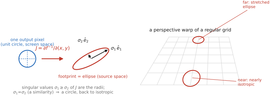
The canonical offender is exactly the floor we opened with: a checkerboard plane rendered in perspective, or rectified to perspective. Near the camera one pixel covers one tile and $\rho\approx1$; toward the horizon one pixel covers many tiles in depth but only one across, and $\rho$ climbs into the tens or hundreds. That is where every isotropic filter visibly fails, and the failure is not a matter of taste but of geometry. A round kernel has one radius, and the footprint has two very different ones. The fix is to make the kernel an ellipse that matches the footprint: the L16 prefilter, now carrying an orientation. Figure 11.2.2⛶ fullscreen shows the three outcomes side by side on a genuine perspective checkerboard.

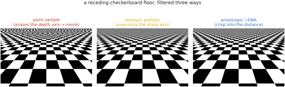
For example, suppose the inverse warp stretches one output-pixel distance into four source-pixel distances horizontally and one vertically. A circular source filter wide enough for the horizontal compression also averages too much vertically. A filter narrow enough to retain the vertical detail leaves horizontal frequencies that can alias. An elongated footprint expresses the two requirements separately. Rotate the warp and the long axis rotates as well; a scalar level-of-detail value cannot describe both its orientation and its unequal axis lengths. The ellipse is a convenient approximation based on a circular filter footprint and a local linearization, rather than the exact image of a square pixel under an arbitrary nonlinear warp.

11.2.2 EWA: the elliptical weighted average🔗⧉

The gold-standard answer is to weight each source texel inside the footprint by an elliptical Gaussian matched to the ellipse, then normalize. This is the elliptical weighted average (EWA), due to Greene & Heckbert (1986) and developed in full in Heckbert's 1989 thesis. It is precisely the reconstruct-and-prefilter convolution of Chapter 11.1, Warping with the kernel finally allowed to be non-round: the round Gaussian of the isotropic prefilter becomes an anisotropic Gaussian whose covariance is the footprint covariance $\Sigma=JJ^{\top}$.

What makes EWA practical, and not merely correct, is that an ellipse is the level set of a quadratic. Write the Mahalanobis form

where $\mathbf u=(u,v)$ is the offset of a texel from the footprint center. Then a texel lies inside the footprint exactly when $Q\le F$ (the cutoff $F$ fixes how many standard deviations of the Gaussian we keep), and its weight is the elliptical Gaussian $w=\exp(-\tfrac12 Q)$. So the whole filter is a tidy loop: walk the axis-aligned bounding box of the ellipse, accumulate $w\cdot\text{texel}$ wherever $Q\le F$, and divide by $\sum w$. The conic both tests membership and supplies the weight (Figure 11.2.3⛶ fullscreen).

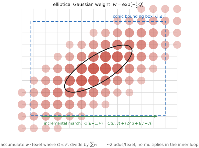
That incremental update is the useful part and the reason EWA was already practical in 1986. Because $Q$ is a quadratic in the integer texel coordinates, its first difference along a scanline, $Q(u{+}1,v)-Q(u,v)=2Au+Bv+A$, is merely linear, and that quantity's own increment is the constant $2A$. So you carry two running sums, $Q$ itself and its per-step increment, and advance both by addition. The per-texel cost collapses to about two adds and one table lookup for the exponential; there are no multiplies in the inner loop at all.

The cost that does bite is the ellipse area, which is proportional to $\sigma_1\sigma_2$ and explodes at grazing angles where $\sigma_1$ runs away. Two guards keep it bounded. First, run EWA on a MIP pyramid: pick the pyramid level at which the minor axis is about one texel, and at that level the remaining sample count is governed mainly by the anisotropy: the prefiltered pyramid has already done the across-axis averaging for you, so EWA only has to integrate along the major axis. Second, cap anisotropy by broadening the minor-axis support to at least $\sigma_1/\rho_{\max}$ and select a compatible pyramid level. This trades extra blur for bounded work while retaining the major-axis antialiasing footprint. Shortening the major axis instead would trade away antialiasing. Pyramid filtering, finite support and level selection make the result an approximation.

11.2.3 Feline and anisotropic MIP probing: EWA on a GPU budget🔗⧉

Integrating the entire ellipse is more than real-time rendering can afford per pixel, so hardware uses a clever approximation. The move, due to McCormack, Perry, Farkas & Pijewski (1999), Feline for Fast Eliptical Lines, stops integrating the area and integrates a line instead: approximate the footprint ellipse by a row of circular probes strung along its major axis. Each probe is an ordinary trilinear MIP sample sized to the minor axis $\sigma_2$, so it averages correctly across the ellipse, reusing the prefiltered pyramid, and the $N$ probes, spaced along the major axis $\hat e_1$ and summed with Gaussian weights, cover the ellipse's length. The ellipse's area integral becomes a short sum of cheap point queries (Figure 11.2.4⛶ fullscreen).

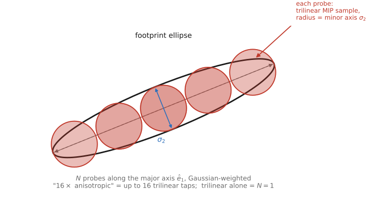
Two limiting cases make the design clear. With $N=1$ the line collapses to a single probe, which is plain trilinear filtering: an isotropic footprint that must choose one MIP level for both axes, and so over-blurs along the minor axis whenever the ellipse is elongated. As the ellipse lengthens, $N$ grows with the ratio of major to minor axis, but every probe still costs one trilinear lookup no matter how large the footprint is, because the MIP level absorbs the width. The cost per output pixel is therefore proportional to the anisotropy ratio, not to the footprint's area, which is what makes the method affordable in real time.

Hardware anisotropy settings bound a quality/cost tradeoff, but do not specify an exact number or arrangement of trilinear probes across vendors. Feline illustrates a probing strategy McCormack et al. 1999; treat it as an algorithm, not a literal description of every GPU implementation.

11.2.4 Other footprint integrators: summed-area tables and ripmaps🔗⧉

EWA and Feline buy arbitrarily oriented anisotropy. Two older structures buy the cheaper, axis-aligned kind, and they are worth knowing both for where they still live and for the precise way they fall short.

A summed-area table (SAT), due to Crow (1984), precomputes the integral image $S$, the running sum of all pixels above and to the left of each location. With $S$ in hand, the average over any axis-aligned box is just four corner lookups,

an $O(1)$ operation for any box size with no pyramid at all. The catches are two. It handles axis-aligned rectangles only. There is no way to tilt the box, so it can never match a rotated footprint ellipse, only an upright one. And the partial sums grow enormous (they accumulate the whole image), so a SAT is badly precision-hungry and wants wide integer or float storage. A ripmap is the complementary idea: an anisotropic MIP-map Williams 1983 that is separately pre-shrunk in $x$ and in $y$, forming a 2-D grid of levels indexed by $(\text{LOD}_x,\text{LOD}_y)$, so an axis-aligned anisotropic footprint reads one matching level directly. It too is blind to rotation, and it approaches 4× the base-image storage, versus 4/3× for an ordinary two-dimensional MIP pyramid, or about 3× the pyramid storage (Figure 11.2.5⛶ fullscreen).

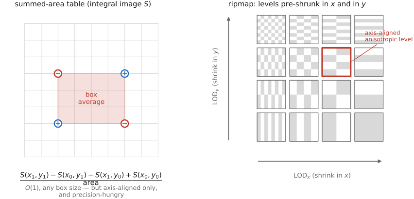
Where each sits is then clear. SATs and ripmaps give axis-aligned anisotropy cheaply; EWA and Feline give arbitrarily oriented anisotropy, which is the case that actually arises under perspective, where the receding-floor ellipse points along whatever direction the depth gradient happens to take. So in practice GPU texture units use multi-probe schemes in this spirit for texturing, while summed-area tables survive less in texture filtering than in other integral-image uses, such as box filters, Viola–Jones face detection Viola & Jones 2001, and local-contrast normalization, wherever a fast axis-aligned box average is the whole job.

11.2.5 Footprint estimation, clamping, and when to reach for it🔗⧉

Everything above assumes we know the footprint, which means knowing the Jacobian $J$. Happily it usually comes for free. In a renderer, screen-space derivatives of the texture coordinates ($\partial u/\partial x$ and the rest, exposed on the GPU as the ddx/ddy instructions) are the two columns of $J$ directly. In an image warp it is the local linearization of $f^{-1}$ that you are already evaluating to do the inverse lookup. Either way, two derivative vectors give the $2\times2$ matrix $J$, from which $\Sigma=JJ^{\top}$ and the ellipse follow. And the chapters join up exactly at the similarity case: for pure minification with no warp, $J$ is a scaled identity, $\Sigma$ is a circle of the downscale radius, and EWA degenerates back into the isotropic L16 prefilter of Chapter 11.1, Warping. The two treatments are one continuous story, with this chapter the strictly more general end.

Use enough minor-axis support for reconstruction. To cap the anisotropy while retaining major-axis antialiasing, one conservative choice broadens the minor radius to at least $\sigma_1/\rho_{\max}$; this trades extra blur for bounded anisotropy. Simply shortening the major axis can reintroduce aliasing. A ratio cap alone does not bound absolute footprint area; prefiltered pyramid levels control that cost. At visibility boundaries or rapidly changing warps, split or adapt the footprint rather than assuming one Jacobian covers the whole pixel.

Finally, the plain decision aid, because this machinery is not always worth its cost. A gentle affine, a panorama reprojection, a mild lens-distortion correction: these are usually close enough to similarities that the isotropic L16 prefilter (a MIP-map plus trilinear) is sufficient, and EWA adds cost with little visible gain. Check the Jacobian rather than the name of the warp: a panorama reprojected far from its center can still produce strongly elongated footprints. Save the anisotropic machinery for strong perspective, swirls, and grazing-angle minification, anywhere the footprint ellipse gets long and one axis would otherwise alias. That is precisely the rectifier's non-uniform Jacobian in Chapter 11.6, Perspective distortion and its correction, and the receding-ground case we opened with: the warps where the floor crawls unless you average along the ellipse.

One last connection points forward. The same elliptical Gaussian runs in reverse for point-based rendering: rather than gathering source texels into an output pixel, Zwicker et al.'s EWA splatting forward-splats each point into the image as an elliptical-Gaussian footprint and accumulates. It is the antialiasing dual of EWA texture filtering, gather versus scatter of the very same kernel, and a direct ancestor of today's Gaussian-splatting view synthesis, where a scene is a cloud of anisotropic Gaussians splatted into each new view. (Cross-reference the novel-view-synthesis material.) The ellipse you matched to a pixel's footprint here is the same ellipse a splat paints there.

11.2.6 Jacobians of common warps🔗⧉

Because the footprint is read straight off the Jacobian $J=\partial f^{-1}/\partial(x,y)$, it helps to have the Jacobians of the warps that actually come up. Each is a small $2\times2$ matrix, cheap to evaluate per pixel once written down. Below, $\ell$ is the focal length.

Homography. With $f(x,y) = \big(\tfrac{ax+by+c}{gx+hy+1},\ \tfrac{dx+ey+f}{gx+hy+1}\big)$, write $w = gx+hy+1$ and the outputs $x' = (ax+by+c)/w$, $y' = (dx+ey+f)/w$. Then

For the inverse-warp Jacobian the resampler needs, apply the same formula to the entries of $H^{-1}$.

Cylindrical panorama. Projecting onto a cylinder, $(\theta, v) = \big(\arctan\tfrac{x}{\ell},\ \tfrac{y}{\sqrt{x^2+\ell^2}}\big)$,

Spherical. With $(\theta,\varphi) = \big(\arctan\tfrac{x}{\ell},\ \arctan\tfrac{y}{\sqrt{x^2+\ell^2}}\big)$, let $r=\sqrt{x^2+\ell^2}$ and $s=\sqrt{x^2+y^2+\ell^2}$; then

Mercator. From longitude and latitude, $u=\lambda$ and $v=\ln\tan\!\big(\tfrac{\pi}{4}+\tfrac{\varphi}{2}\big)$. This angular-coordinate Jacobian is diagonal with $\partial v/\partial\varphi=\sec\varphi$, the latitude stretch that diverges at the poles. For a camera-image warp, compose it with the camera-to-spherical Jacobian; the complete image-coordinate Jacobian is generally not diagonal.

When the algebra is ugly, do not do it by hand. A symbolic package (SymPy, Mathematica) differentiates the warp once at authoring time and emits the closed-form entries to paste in; automatic differentiation (JAX, PyTorch, or a dual-number pass) evaluates $J$ exactly at each pixel with no formula at all. Both earn their keep when the warp is learned or composed and has no tidy expression.

Or just use finite differences. $J$ is only a $2\times2$ matrix, and the warp is already being evaluated at neighboring pixels, so a one-pixel central difference reads its two columns off samples you are taking anyway,

These are central finite differences of the warp. GPU derivatives typically use neighboring fragment values and are not exactly this stencil. Their validity also depends on execution and discontinuity handling. Convert normalized texture coordinates to source-pixel units before interpreting axis lengths.