10.5 Matting Laplacian⧉
Hair against a background needs fractional coverage, not just a binary selection. Closed-form matting estimates that coverage using a local affine relation between color and alpha Levin, Lischinski & Weiss 2008 (closed-form matting). Like colorization it leads to a sparse quadratic solve, but the matrices are different.
That question is harder than it first sounds, and the result is a soft, fractional mask that lets you lift a person off their background and drop them onto another, hair and all, with no telltale fringe. So we begin where the difficulty lives, in the equation that defines the problem.
10.5.1 The matting problem: compositing, and why it is under-determined⧉
At boundaries, unresolved coverage, defocus or partial transparency can mix foreground and background contributions. The standard compositing model writes this mixture in a common linear-light space:
This is the compositing equation, and the weight $\alpha \in [0,1]$, the opacity or alpha, is exactly what we want. Where the object solidly covers the pixel, $\alpha = 1$ and $I = F$; where only background shows, $\alpha = 0$ and $I = B$; and in between, $\alpha$ is a genuine fraction. Recover $\alpha$ at every pixel (the alpha matte), together with the foreground color $F$, and you can re-composite the object by running the equation forwards with a different $B$ (Figure 10.5.1).
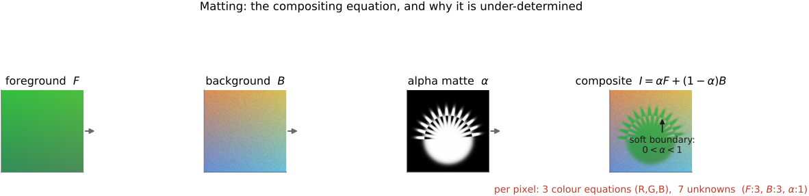
Now count. At each pixel the camera hands us $I$, three numbers, R, G and B. But the equation we must invert has seven unknowns hiding behind them: three for $F$, three for $B$, and one for $\alpha$. Three equations, seven unknowns, per pixel. The problem is not merely hard; it is wildly under-determined, hopeless to solve pixel by pixel. Like every ill-posed recovery in this book, it can only be pinned down by a prior (a model of what plausible solutions look like) together with a few marks from the user. That is the L7.8 lesson again (the prior is not optional, Chapter 7.5, Image priors); the rest of the chapter is the story of which prior, and how cheaply it lets us solve.
Before that, one point of principle comes first, because it is the whole reason matting earns a chapter separate from segmentation. The alpha we are solving for is soft, a continuous number, not a hard zero-or-one label. This matters wherever an object's boundary is not a clean line: hair, fur, a smoky edge, motion blur, the rim of a glass. There a single pixel contains both foreground and background, and the only truthful answer is a fraction. A hard segmentation, the graph-cut Boykov & Jolly 2001 and GrabCut Rother et al. 2004 machinery of the next chapter, Chapter 10.9, Seam optimization, slices each pixel firmly into object or background. It simply cannot represent a wisp of hair that is sixty-percent strand and forty-percent sky. Matting can. (The two meet in the middle: GrabCut's border-matting step, which softens its hard cut into a narrow anti-aliased band, is a lightweight precursor to the full matte we build here.)
10.5.2 The color-line assumption: α becomes linear in color⧉
The prior that rescues matting is a statement about color in small windows, and we have already met it. In Chapter 7.5, Image priors (§Linear color models) we plotted the pixels of a little image patch in RGB space and found that they do not scatter every which way: they lie, to good approximation, on a short line segment: the color-line model. The reason is simple. A small enough patch usually contains at most one or two materials under gently varying shading, so its colors are a linear mixture of a few endpoints, collapsing onto a one-dimensional line in the color cube. We treat that observation as known here and put it to work; the figure recalls it (Figure 10.5.2).
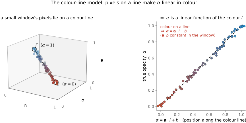
Here is what that buys us in the matting problem specifically. Suppose that inside a small window the foreground color $F$ and the background color $B$ are each roughly constant and distinct. Then the compositing equation $I = \alpha F + (1-\alpha) B$ says every pixel of the window sits on the line through $B$ and $F$, and a pixel's opacity $\alpha$ is nothing but how far along that line it has traveled: zero at the $B$ end, one at the $F$ end. Position along a line is an affine function of position in space, so
where the three-vector $\mathbf{a}$ and the scalar $b$ are the same for every pixel $i$ in the window. This is the single structural assumption behind closed-form matting (Levin, Lischinski & Weiss Levin, Lischinski & Weiss 2008 (closed-form matting)): within a small window, $\alpha$ is a linear function of the image colors. It is the color-line prior of Chapter 7.5, Image priors, stated as a working hypothesis about the unknown we want.
This is the right prior because it turns an intractable per-pixel color-matching problem into a clean linear statement, and, as we are about to see, a linear relationship between $\alpha$ and $I$ is exactly what lets us make the unknowns $F$ and $B$ disappear.
10.5.3 Closed-form matting: the matting Laplacian⧉
Within window $w_k$, penalize departures from a local affine color model, with ridge regularization:
Eliminating the local coefficients analytically leaves a quadratic in alpha. This uses the affine prior; it does not solve the unconstrained physical foreground/background problem.
The original nonlinear, seven-unknowns-per-pixel problem has collapsed into a single quadratic form in the one quantity we care about. The matrix $L$ at its heart is the matting Laplacian.
Here is what the color-line assumption does for us, because the algebra can obscure it. The compositing equation couples three unknowns per pixel ($F$, $B$, $\alpha$) and the color ones, $F$ and $B$, are both the most numerous (six of the seven) and the least interesting (we only want $\alpha$). A general nonlinear prior on $F$ and $B$ would leave us alternating: fix $\alpha$, estimate the colors; fix the colors, estimate $\alpha$; repeat. The color-line assumption makes $\alpha$ a linear function of the colors inside each window, and a linear relationship can be solved out in closed form: the best $\mathbf{a}, b$ (and hence the role of $F$ and $B$) for any given $\alpha$ is a least-squares formula, which we substitute back rather than iterate on. The six nuisance unknowns vanish analytically, and a problem that looked like alternating optimization becomes a single quadratic in $\alpha$. The matting Laplacian is precisely the residual of that elimination: it is what the windowed least-squares fit leaves behind once the colors are gone.
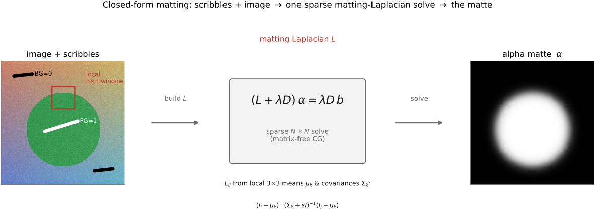
What is $L$? It is a large, sparse $N \times N$ matrix, with one row and column per pixel, and its entries are assembled from purely local statistics: for each small window $w_k$ (a $3 \times 3$ patch, in practice), compute the mean color $\mu_k$ and the color covariance $\Sigma_k$ of the pixels in it, and let those drive the affinity between any two pixels $i$ and $j$ that share the window. The entry $L_{ij}$ is built from a term of the form
Here $n_k=|w_k|$, $\mu_k$ and $\Sigma_k$ are the population mean and covariance of the RGB values in the window, $I_3$ is the 3×3 identity, and $\delta_{ij}$ is one when the indices agree. This scale of regularization matches the preceding window energy. The matrix is symmetric positive semidefinite with a constant null mode before constraints.
The local color model connects matting to guided filtering He et al. 2010. It does not make the matting Laplacian identical to a bilateral graph or the colorization normal matrix; its off-diagonal structure need not correspond to nonnegative pairwise affinities.
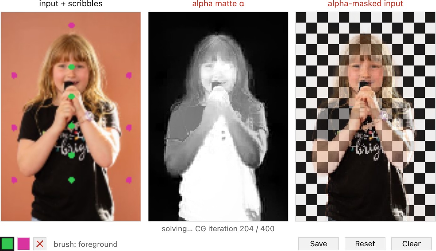
With $L$ in hand, the recovery is the colorization recipe verbatim. The user scribbles a few strokes: some over the object, marking definitely foreground ($\alpha = 1$); some over the background, marking definitely background ($\alpha = 0$). Those marks are the data term. Minimize the energy $\alpha^{\!\top} L \alpha$ subject to them, and, because the energy is quadratic and the constraints are linear, the minimizer is the solution of a single sparse linear system:
where $D$ is a diagonal matrix flagging the scribbled pixels, $b$ holds the values the user painted there ($0$ or $1$), and $\lambda$ is a large weight that turns the scribbles into near-hard constraints. One solve, and the opacity floods out from the marks along high-affinity color-line paths to fill the whole image, exactly as color flooded out in the previous chapter. The reader can drive the whole loop, scribble and solve, in the interactive demo (Figure 10.5.5).
The contrast with what came before in the matting literature is the headline. Earlier methods (next section) estimated the foreground and background colors $F$ and $B$ explicitly, alternating between guessing colors and guessing opacity, iterating to convergence. Closed-form matting does none of that. Because the local affine coefficients were eliminated analytically, there is no alternating F/B estimation in this formulation. There is one quadratic energy and one linear system, which can itself be solved iteratively. That is what "closed-form" means, and it is the whole appeal.
The operator has one row per pixel, but is sparse. Store a sparse matrix or apply an equivalent local operator; avoid a dense matrix. A solver and preconditioner must respect the constrained nullspace. Runtime depends on resolution, conditioning and implementation.
The shared computational pattern is a sparse constrained quadratic solve. The prior, matrix coefficients and nullspace determine the behavior of each method.
An unconstrained quadratic solve need not keep alpha in [0,1]. State whether the implementation clips afterward or solves with bounds. Re-compositing also needs foreground color estimation or decontamination where the old background contributed to RGB.
The elimination is the useful step. For a tentative opacity field, ask which affine function of the observed colors best fits its values in one window. That is a small regularized least-squares problem in the local color coefficients. Substituting its optimum into the window's cost removes those local coefficients, leaving a quadratic expression in opacity. Sum the window costs and add the foreground/background constraints to obtain one global system. The local algebra removes the need to alternate explicit foreground and background color estimates with opacity estimates; it does not remove the need to solve the resulting large linear system, potentially iteratively.
10.5.4 Spectral matting: eigenvectors of the matting Laplacian⧉
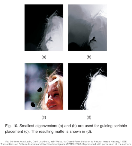
Small-eigenvalue eigenvectors describe opacity variations that cost little under the local affine model. Spectral matting (Levin, Rav-Acha & Lischinski Levin, Rav-Acha & Lischinski 2007 (spectral matting)) takes the matting Laplacian and, instead of solving a scribble-constrained system, simply computes its smallest eigenvectors. These turn out to be soft, fuzzy fragments of the image, which the authors call matting components, each one a partial alpha-like piece of the picture (Figure 10.5.7).
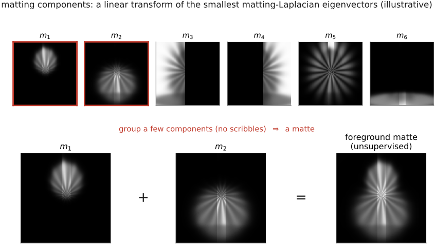
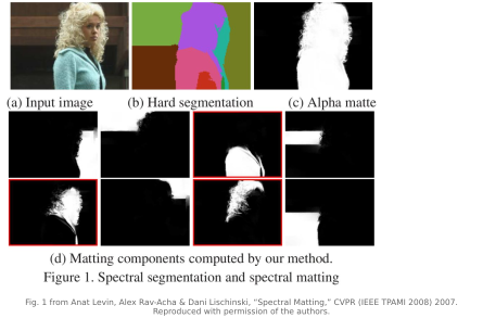
Spectral matting first extracts candidate components from eigenvectors. Selecting or grouping those components into a desired foreground remains a separate step and may use interaction or an additional criterion. Eigenvectors alone do not identify which object the user intends to cut out.
The move should feel familiar, because it is the same move that the next chapter makes for segmentation. Normalized cuts (Chapter 10.9, Seam optimization) partitions an image by computing the smallest eigenvectors of a graph Laplacian built from a pixel-affinity matrix. Spectral matting computes the smallest eigenvectors of the matting Laplacian. It is the same spectral idea (read an image's natural grouping off the small eigenvectors of an affinity Laplacian) with the matting Laplacian standing in for the graph Laplacian. The only difference in spirit is hard versus soft: normalized cuts thresholds its eigenvector into a crisp two-way partition, while spectral matting keeps its components continuous, so the result is a soft matte rather than a hard boundary. One Laplacian, two readings: solve it against scribbles (closed-form matting), or read its spectrum (spectral matting).
10.5.5 An alternative matting Laplacian⧉
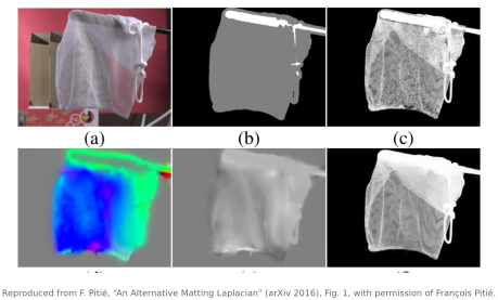
The matting Laplacian of Levin, Lischinski & Weiss 2008 (closed-form matting) is one particular way to package the color-line idea into a matrix, and it is not the only useful one. François Pitié Pitié 2016 (alternative matting Laplacian) revisits the derivation and offers an alternative matting Laplacian, a reformulation that exposes the matting parameters more flexibly and, in particular, handles upsampling better. The practical win is the familiar coarse-to-fine trick: solve for a matte cheaply at low resolution, then upsample it to full resolution guided by the high-resolution image, with the reformulated Laplacian giving a cleaner, sharper refinement than naively re-solving at full size. It is the matting cousin of the joint-bilateral and guided upsampling we met in Chapter 10.1, Bilateral filtering (do the expensive solve small, carry the edges from the big image) and a reminder that "the matting Laplacian" names a family of closely related operators, not a single frozen formula.
10.5.6 Beyond matting: spatially-varying white balance⧉
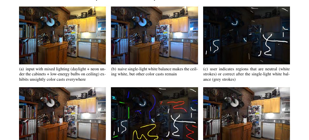
The clearest proof that the matting Laplacian is a general tool, not a matting trick, is an application that has nothing to do with cutting out objects. Recall the white-balance problem from the ISP: a single global multiply neutralizes one illuminant. But a real room often mixes two, warm tungsten from a lamp and cool daylight from a window, in proportions that vary from pixel to pixel. No global gain can fix both at once. Hsu et al.'s User-guided White Balance for Mixed Lighting Conditions Hsu et al. 2008 reframes this as a soft-segmentation problem solved with the matting Laplacian: the unknown per-pixel "alpha" is now the mixing fraction between the two illuminants, and the same color-line affinity that pulls a foreground matte propagates that fraction smoothly within surfaces and snaps it at edges, starting from a handful of user strokes marking neutral regions. With the per-pixel mixture in hand, each pixel can be white-balanced by its own blend of the two illuminant gains. Same operator, same one sparse solve; only the meaning of the unknown changed. Opacity became illuminant fraction (Figure 10.5.9).
Where matting goes from here. The methods that now dominate practice, the sampling-based classics (Bayesian and optimized-color-sampling matting), the studio special case of blue-/green-screen keying, and above all the learned and generative successors (trimap-based deep matting, background-free real-time video matting), are taken up later, in the SINGLE IMAGE part's Part 19, Layers, transparency, compositing, and matting. Carry forward the affinity at the center of this method. The matting Laplacian's color-line graph is a tool well beyond matting: the same operator drives colorization, segmentation, and edge-aware editing, and it persists inside the learned methods, as a loss term or a refinement stage that enforces the color-line structure a network might otherwise miss. The hand-built affinity did not vanish when the networks arrived; it moved inside them. Understanding it is still understanding what these problems are.