9.3 Image metrics⧉
A denoiser should agree with a clean capture. A compressor should preserve its input. An alignment algorithm should put corresponding structures in the same place. Each needs a numerical measure, but the errors that matter differ. A one-pixel displacement is serious for registration even when it barely changes the appearance of a photograph viewed alone.
This chapter distinguishes pixel fidelity, structural similarity, and predicted visibility. None measures every aspect of image quality or replaces evidence about people's preferences. Chapter 9.2, The expert's eye as evaluation and Chapter 9.4, Towards meaningful user studies cover the complementary questions.
9.3.1 Full-reference vs. no-reference⧉
A full-reference measure compares a candidate with a specified reference: an uncompressed source, a synthetic clean image, or a carefully acquired high-quality capture. The reference need not be perfect. A long-exposure “clean” image may have motion blur; a burst average may contain alignment errors. For resampling, the high-resolution image must first be related to the output's sampling grid before a pixelwise comparison is meaningful.
A no-reference measure scores one image using a model of expected image statistics or learned quality judgments. It can help find blur or compression damage when no reference exists: a phone deciding that a frame is too blurry to keep, or a streaming service monitoring quality across millions of streams. It can also penalize intentional grain or shallow depth of field, or favor a sharp hallucination. Validate it on the kinds of images and defects your application produces.
For either regime, specify the input domain. Linear raw error measures something different from error after white balance, a tone curve, and an output encoding. Use the same registration, crop, masks, channel order, and preprocessing for every method. Do not independently normalize each output unless invariance to that normalization is part of the question. Masking borders or correcting exposure can remove the very errors a benchmark is meant to detect.
9.3.2 Why not just L2?⧉
Flatten two aligned images into $N$ scalar samples, counting each channel separately. Their mean squared error is
Subtract corresponding samples, square, and average. This is the squared Euclidean distance divided by the sample count. Convert unsigned integer samples to a suitable signed or floating-point type before subtracting; otherwise subtraction or squaring may overflow.
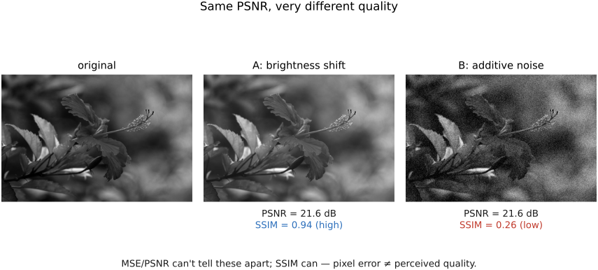
MSE treats equal squared errors equally regardless of their location or structure. It can assign the same score to a brightness change and a conspicuous block artifact. A small translation can give a large error along edges even if the displaced photograph looks acceptable in isolation. The displacement is still visible in an aligned toggle and may be unacceptable for a geometric task.
Squaring gives large residuals disproportionate weight. Mean absolute error, $N^{-1}\sum_i |I_i-J_i|$, grows linearly with their magnitude and is less sensitive to outliers. Both are useful fidelity objectives; neither accounts for the spatial visibility of an error.
Squared error is smooth and mathematically convenient, and strongly penalizes large residuals. For a linear model, unconstrained least squares leads to a linear system. A neural network trained with the same loss remains a nonlinear optimization problem. Under squared error, the optimal prediction of an uncertain target is its conditional mean, which explains the averaging discussed in Part 13, Denoising.
MSE remains useful despite those limits. It is inexpensive and differentiable, with gradient $2(I_i-J_i)/N$ with respect to the candidate sample $I_i$. That gives an optimizer a direct, stable signal for reducing pixel error. Choosing it as a loss commits to that objective; it does not establish that equal loss improvements have equal perceptual value.
9.3.3 PSNR⧉
Peak signal-to-noise ratio expresses the same error in decibels:
Here $L$ is the fixed reference range: $1$ for normalized samples in $[0,1]$, or $255$ for 8-bit samples. It is not each image's measured maximum. For HDR values without a shared finite range, specify a normalization or use a measure designed for the intended luminance conditions. PSNR is not the sensor SNR discussed in Chapter 2.8, Noise, signal-to-noise ratio and dynamic range: the denominator here includes any discrepancy from the reference, including bias, blur, and registration errors.
Higher PSNR means lower MSE at the same $L$; zero error gives infinity. Halving MSE adds about 3 dB. There is no universal threshold for an acceptable image. Scores depend on the scene, encoding, crop, and degradation.
Be explicit about aggregation. Averaging image PSNRs differs from pooling squared errors and converting once, because the logarithm is nonlinear. For equal-sized images with MSEs $0.001$ and $0.01$ at $L=1$, the mean PSNR is 25 dB, while the PSNR of their mean MSE is about 22.60 dB. Report the convention and inspect the distribution, not only its mean.
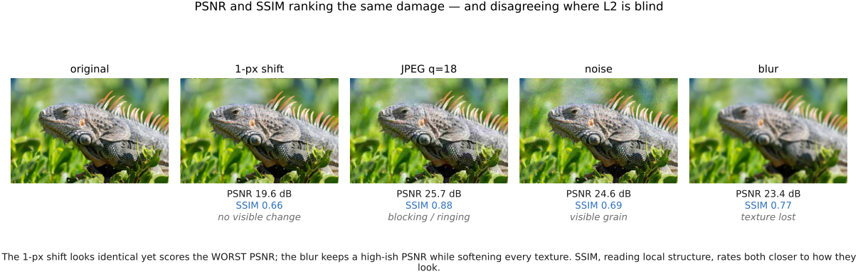
Linear RGB is useful for radiometric fidelity; a specified output encoding measures errors after rendering. Color differences such as $\Delta E$ in CIELAB address a different question, under a stated white point and viewing model; see Chapter 4.5, Advanced color: opponents, perceptually-uniform, and preferred. They do not account for spatial structure or automatically make an image-quality benchmark better. Do not apply an RGB PSNR peak to Lab channels and call the result comparable.
9.3.4 SSIM⧉
Structural similarity (SSIM) Wang et al. 2004 compares local brightness, contrast, and correlation. For windows centered at the same location in the two images, a common form is
The means $\mu_I,\mu_J$ describe local brightness; the variances $\sigma_I^2,\sigma_J^2$ describe contrast; the covariance $\sigma_{IJ}$ describes agreement after subtracting the means. The positive constants $C_1,C_2$ stabilize nearly flat or dark windows. Identical windows score one. Scores can be negative, particularly when local patterns are anticorrelated. Wang et al.'s formulation specifies the window and constants needed to reproduce a score.
SSIM is a map before it is a number. Because the window slides across the image, what SSIM produces first is a per-pixel structural-similarity image. Its displayed values indicate local agreement under the chosen visualization. The single "SSIM" value people quote is just that map's average. The map retains spatial information, because it localizes the damage in a way a scalar never can.
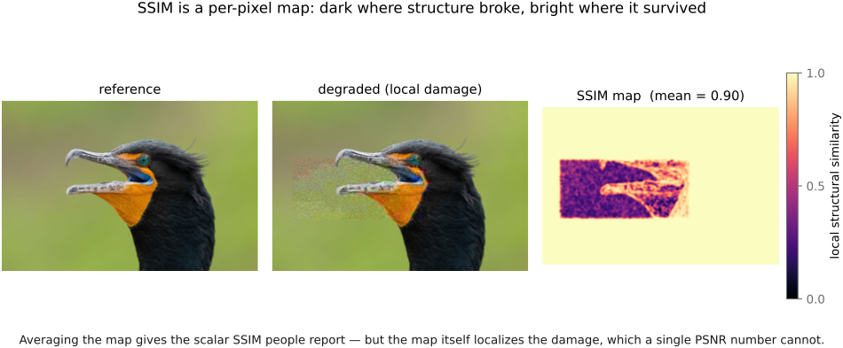
SSIM adds useful spatial information but remains sensitive to window size, scale, and alignment. A luminance-only implementation misses purely chromatic errors. Multi-scale SSIM compares several resolutions. Record the implementation, input range, channel handling, window, and border convention; the name alone is not a complete evaluation protocol.
9.3.5 VDP and HDR-VDP⧉
A visible differences predictor (VDP) Daly 1993 models contrast sensitivity and masking to estimate the visibility of differences. The same residual may be conspicuous in a smooth sky and hidden in a textured surface. Visibility varies gradually with contrast and viewing conditions; a threshold summarizes a chosen detection probability, rather than a sharp boundary below which nobody can see anything.
HDR-VDP-2 Mantiuk et al. (HDR-VDP) includes adaptation across luminance levels and provides visibility and quality predictions. It needs the display interpretation: physical luminance and angular image resolution, which depends on screen size and viewing distance. A raw array spanning many stops is not sufficient. Treat its output as a model prediction under those conditions, not a probability that any particular person will notice a defect in ordinary viewing. See the HDR-VDP-2 paper.
Consider adding the same small oscillating error to a smooth wall and to dense foliage. A pixelwise squared-error measure can assign them the same score. A visibility model treats them differently because the foliage can mask an error whose frequency and orientation overlap its texture. Now view both images from farther away: sufficiently fine errors become harder to resolve. Change display luminance and adaptation, and the visibility can change again. This is why a visual difference predictor needs viewing conditions as well as the two arrays. Its output estimates detection under its model and calibration; it does not impose a universal hard boundary between visible and invisible errors.
9.3.6 Learned metrics⧉
Learned perceptual measures compare neural-network features instead of raw pixels. LPIPS evaluates feature differences calibrated against judgments of distorted image patches; the authors' project provides the model and evaluation data. DreamSim targets broader visual similarity using human judgments of synthetic image triplets, as described in its project page. Their training questions differ, so their scores need not agree.
Use the prescribed network, checkpoint, input normalization, and resolution. A metric that tolerates a small structural change may be useful for similarity but unsuitable when preserving that structure is essential. Test its behavior on your own degradation family before treating a small improvement as evidence of better quality.
LIVE, TID2013, and KADID-10k provide human judgments for validating image-quality measures; see Chapter 45.16, Datasets. Check which distortions and viewing conditions a dataset covers before transferring its conclusions to camera raw data or generated images.
Differentiable feature distances can also serve as training losses, as developed in Deep learning#Learned perceptual metrics and losses. They can favor plausible texture over exact recovery. A sharper result therefore does not by itself establish that the recovered detail was present in the scene.
The feature representation is itself an important observation: a network trained for recognition can contain information useful for judging texture and image structure, even though its original task was not to predict visual differences. Learned similarity methods select, normalize, and sometimes calibrate those features for a different question. The resulting metric inherits both the representation’s useful invariances and its blind spots. A recognition feature that deliberately ignores a change can be a poor test when preserving that change is the reconstruction task.
9.3.7 The right metric depends on the task⧉
Choose the measure from the claim. For agreement with a known image, report a clearly specified pixel-fidelity measure. For artifact visibility, use a perceptual model suited to the display and distortions. For preference or task performance, collect the corresponding judgments or behavior. Complement scalar scores with maps, image examples, and failure frequencies.
Optimizing a score can improve what it measures while exploiting what it ignores. The score does not automatically become useless, and evaluating a training loss on held-out data still measures generalization of that objective. But it is weak independent evidence for a broader quality claim. Reserve evaluation data, inspect outputs, and use complementary measures or human judgments that match the claim. Repeated tuning against the “held-out” measure makes it another target.
Recap: big lessons of this chapter
Squared error is smooth and mathematically convenient, and strongly penalizes large residuals. For a linear model, unconstrained least squares leads to a linear system. A neural network trained with the same loss remains a nonlinear optimization problem. Under squared error, the optimal prediction of an uncertain target is its conditional mean, which explains the averaging discussed in Part 13, Denoising.
Optimizing a score can improve what it measures while exploiting what it ignores. The score does not automatically become useless, and evaluating a training loss on held-out data still measures generalization of that objective. But it is weak independent evidence for a broader quality claim. Reserve evaluation data, inspect outputs, and use complementary measures or human judgments that match the claim. Repeated tuning against the “held-out” measure makes it another target.