8.10 Auto-exposure and auto white balance⧉
Auto-exposure chooses capture settings and auto white balance estimates a color correction. Both depend on uncertain scene information: a dark object and an underexposed bright object may yield the same measurement, as may a colored surface and colored illumination.
8.10.1 Auto-exposure: metering⧉
A meter estimates scene brightness, then the exposure program chooses shutter duration, aperture, and ISO within constraints. Shutter duration and aperture affect photons collected; ISO affects gain and often the selected exposure. A motion limit, depth-of-field requirement, or highlight constraint can take priority over average brightness.
Average and center-weighted metering. The simplest meter averages the whole frame to one number and exposes so that average is middle gray (see Chapter 5.2, Exposure and capture timing). It is fooled by anything that is not average: a bright sky pulls the average up, so the meter under-exposes and the foreground falls into shadow (the classic backlit-subject silhouette); a snow field reads too bright and is rendered a dingy gray. Center-weighted metering improves the guess by weighting the middle of the frame most, on the assumption that the subject is usually near the center.
Matrix / evaluative metering. Combine measurements from several regions, optionally using focus, face, color, or distance information. Different cameras use different decision rules. Nikon's 3D Color Matrix metering, for example, compares zone brightness and color and the subject distance reported by the lens against a database of reference scenes, which Nikon describes as tens of thousands of photographs; Canon's evaluative metering and other makers' equivalents are cousins. A subject-weighted result may deliberately sacrifice some highlights; an image-wide average does not establish the photographer's intent.
Spot metering is the opposite extreme: meter one small zone and place that tone at middle gray. It hands the photographer exact control over which tone is anchored (the basis of Ansel Adams's Zone System) at the cost of having to choose wisely.
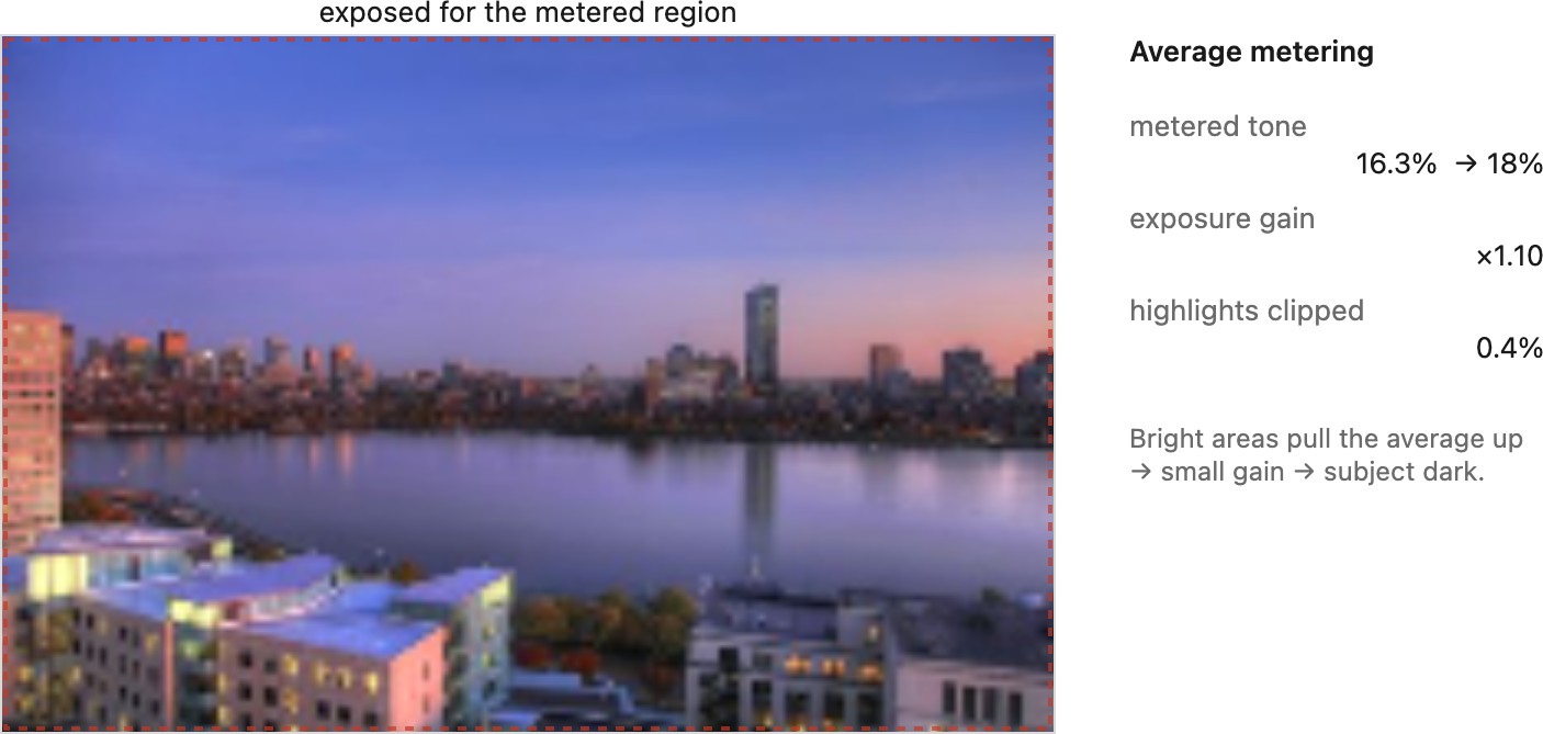
Learned metering. An estimator can learn exposure preferences or use recognized subjects to weight the measurement. Burst pipelines can choose shorter frames to limit motion and saturation, then merge them to reduce noise. Exposure compensation and AE lock remain useful when the intended subject or mood differs from the automatic choice.
For video and preview, both exposure and white-balance estimates also need temporal stability. Damping small frame-to-frame changes reduces flicker, but too much damping delays adaptation after a lighting change.
A zone pattern retains information that an overall average discards. A bright upper region, a darker lower region, and a focused subject between them can suggest backlighting, whereas a uniformly bright frame may be snow or a white wall. Such evidence can guide an exposure decision, but does not settle whether the photographer wants a silhouette. Exposure compensation supplies that missing instruction. The progression from one average to spatial patterns and learned statistics adds evidence about intent without making intent observable directly.
8.10.2 White balance and color constancy⧉
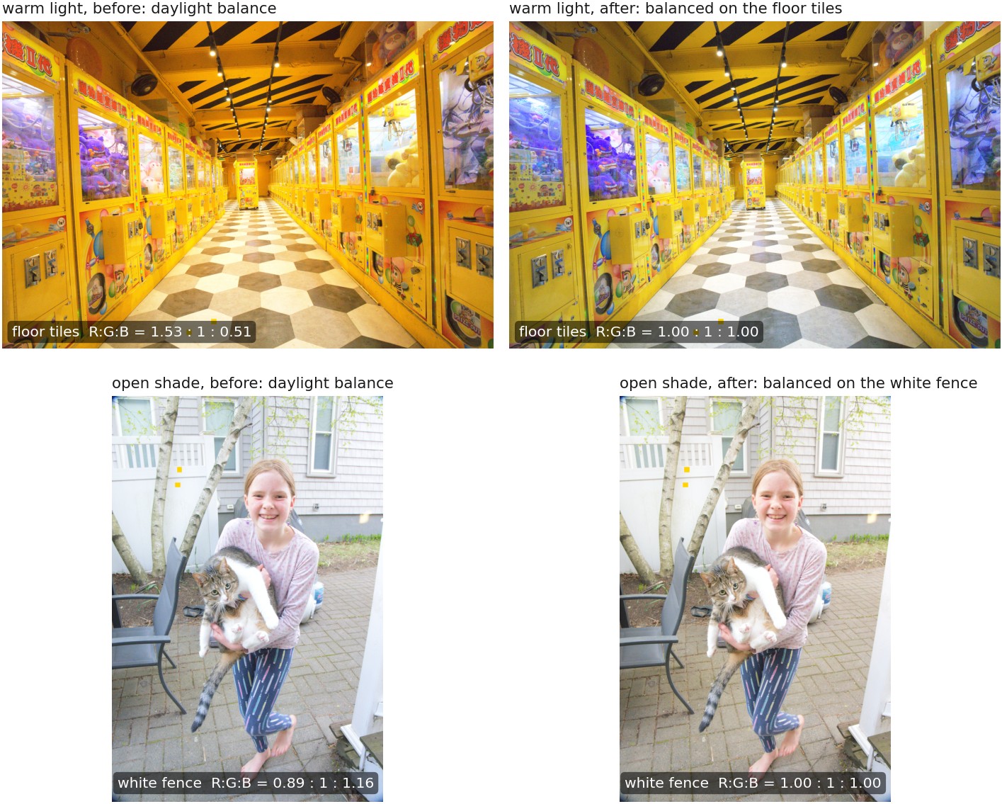
White balance is the harder color-estimation problem. For a simple diffuse surface, the spectrum reaching the sensor depends on the product of the illuminant spectrum and the surface reflectance, so a white shirt under tungsten light sends warm, orange-ish light to the sensor, and the very same shirt under open shade sends cool, bluish light. Yet to a human the shirt looks white under both, because the visual system discounts the illuminant, the color constancy of the perception chapter. A camera has no such automatic constancy; it must estimate the illuminant and divide it out, and that operation is white balance (Figure 8.10.2).
A common approximation uses independent gains in a suitable linear color basis Von Kries:
These gains form a diagonal transform. A known neutral supplies their ratios, with a common scale left for exposure. Camera channels and cone-like adaptation coordinates are different bases; Bradford adaptation is not simply a diagonal scaling in arbitrary RGB. See Chapter 4.2, White balance and white point for that distinction and Land & McCann 1971 for the Retinex connection.
Subtract the calibrated black level before applying sensor-channel gains. Apply them before nonlinear rendering, in the linear basis for which they were estimated. A common scalar exposure commutes with a linear color matrix, but unequal channel gains generally do not: $MD\ne DM$. A gain moved after encoding needs the conjugate operation $g(Dg^{-1}(v))$, not the same numerical multiply. White balance may precede demosaicking; its placement must match the reconstruction and color profile.
8.10.3 White balance on film⧉
Before sensors, white balance was chosen when the film was bought. A color film's three emulsion layers are balanced so that one particular illuminant records as neutral. Daylight film is balanced for about 5500 K, the mix of sun and sky at midday; tungsten film, sold as Type B, for about 3200 K, the color of studio lamps (Figure 8.10.3). Shoot daylight film under household or studio lamps and everything comes out orange, which is the "before" panel of Figure 8.10.2; shoot tungsten film outdoors and everything comes out blue.
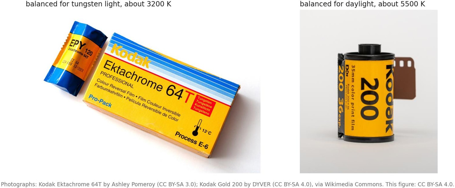
A photographer caught with the wrong film under the wrong light used a conversion filter on the lens. A blue 80A filter lets daylight film record correctly under 3200 K lamps, at the cost of about two stops of light, because it works by absorbing much of the red. An amber 85B lets tungsten film be used in daylight, at the cost of about two thirds of a stop. Photographers reasoned about these filters in mireds, the reciprocal of color temperature scaled by a million,
because a given filter shifts a source by roughly the same number of mireds whatever its temperature. Going from 3200 K (about 312 mireds) to 5500 K (about 182) is a shift of about −131 mireds, which is the 80A's rating, and the 85B is the reverse. Fluorescent tubes, whose spectra are spiky rather than smooth, called for their own filters and often a magenta color-compensating filter to cancel their green cast.
The optical filter is the film-era version of the per-channel gains above, with two differences. It acts on the spectrum before the film records it, so it is a real change to the light rather than a rescaling of recorded numbers, and it costs exposure, which a digital gain does not (though a gain amplifies noise in the channel it raises). And it applies to the whole frame, so a scene lit by two sources, a lamp-lit room with daylight at the window, could not be corrected by any filter on the lens. Film and cinema crews instead filtered the lights themselves, with orange gels on windows or blue gels on lamps, which is the problem Chapter 24.2, Mixed-lighting white balance solves in software.
The two kinds of film also differed in how forgiving they were. A slide is the final image, so a color cast on reversal film is there for good. A color negative is printed, and the printing lab set color filtration for each negative, often with an automatic analyzer, which removed much of a cast after the fact. That printing step was an automatic white balance, run on the negative rather than on sensor data. A digital camera does the same thing per frame, and a raw file defers it entirely, so the choice made at the film counter is now a slider in the editor (Chapter 5.5, Developing and editing a photograph).
8.10.4 Automatic white balance⧉
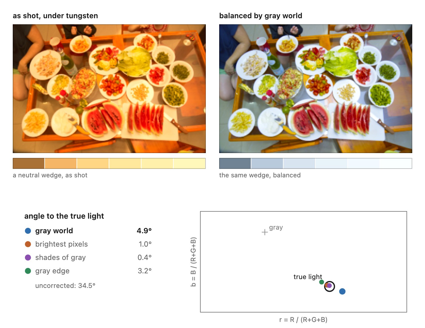
In practice the camera has no labeled neutral patch, so it must guess the illuminant from the image itself: automatic white balance (AWB). The classic assumptions are statistical. Gray-world Buchsbaum 1980 assumes the scene averages to gray, so the channel gains are
Here mean gray can be the average of the three channel means. Use only valid samples and guard near-zero channel means; normalizing the gains to a chosen reference channel separates their common exposure scale. This scales the channels so their means agree (Figure 8.10.4). The bright-pixel (white-patch) assumption (Lee 1986) instead takes the brightest pixels to be a white highlight reflecting the illuminant directly, and balances on those. Both fail in predictable ways: gray-world tips on a scene dominated by one color (a forest, a red wall), bright-pixel tips on a colored specular highlight.
Reject saturated samples and unstable ratios near black when estimating gains. White-patch statistics can select different surfaces in different channels, and a scene need not contain a neutral highlight. Under mixed lighting, one global gain cannot neutralize every region. A neutral reference helps, but white balance cannot reconstruct wavelengths missing from the illumination.
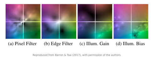
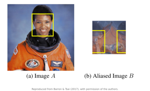
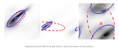
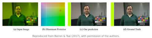
Learned estimators can use richer image statistics than gray-world. FFCC Barron and Tsai, 2017 estimates illumination from a small periodic log-chroma histogram.
For positive linear values, let $u=\log(G/R)$ and $v=\log(G/B)$. Under a global diagonal gain, $u'=u+\log(k_G/k_R)$ and $v'=v+\log(k_G/k_B)$. Thus the model turns illumination into a histogram translation. FFCC uses Fourier-domain filtering, resolves periodic ambiguity, and estimates a posterior rather than only a peak. The periodicity belongs to its histogram representation, not to physical illumination.


Color-constancy sets with ColorChecker ground-truth illuminant; lead with NUS (8 cameras, Cheng, Prasad & Brown 2014 (NUS color-constancy set)), cite Gehler-Shi as the classic baseline (Gehler et al. 2008 (ColorChecker / Gehler-Shi set)). <https://www2.cs.sfu.ca/~color/data/shi_gehler/> · <https://cvil.eecs.yorku.ca/projects/public_html/illuminant/illuminant.html>. See the Chapter 45.16, Datasets appendix.
Test exposure and white balance across a range of skin tones and lighting conditions. A face detector should not imply that every face belongs at one brightness or one color. Historical calibration practices, including Shirley cards, motivate the broader discussion in Chapter 40.2, Ethics of computational photography.
In Chapter 8.13, A raw developer in the browser, White balance is a real Kelvin axis (Planck's law against the CIE observer), and the Auto button on the Tone panel is a learned auto-adjustment: a regression trained on the MIT-Adobe FiveK dataset (Bychkovsky et al. 2011) against expert C, in the app's own slider space. Its ? tells the full story.
This is a localization problem in a representation chosen to simplify the physics. The histogram retains the distribution of channel ratios while discarding their positions in the picture. A learned filter can score possible shifts using distributions seen in training. The estimated two-dimensional shift specifies relative channel gains, leaving their common scale to exposure. The method replaces the single gray-world assumption with a learned statistical model, but surface color and illumination can still admit competing explanations.