8.7 Histograms⧉
A histogram helps judge exposure when glare makes the camera preview hard to read. It shows how many pixels occupy each part of the value range. First check what it measures: most camera histograms describe the rendered preview, so their clipping warnings need not coincide with clipping in the raw sensor data.
8.7.1 The histogram⧉
The histogram of an image is the distribution of its pixel values: for each value (or, in practice, each small bin of values) how many pixels carry it (Figure 8.7.1). That is the whole definition. You sweep the value axis from black (0) to white (1), and at each point you plot a count. A grayscale image gives a single curve; a color image gives three, one per channel, usually drawn overlaid.
A histogram discards position. Shuffle all the pixels and it stays unchanged. This makes it a useful summary of tones, but it cannot tell whether a bright patch is a disposable reflection or an important face. Read it alongside the photograph.
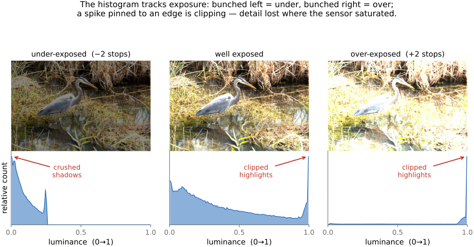
Counts at an endpoint are a reason to inspect that end of the range. They may indicate clipping, but a black background or a uniform white graphic can also produce a spike. An empty part of the range is not necessarily wasted: fog and low-contrast subjects need not contain black and white. Check individual RGB channels as well as luminance, since a saturated red can clip while its luminance remains modest.
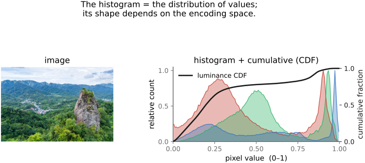
Exposure changes the distribution, but the motion depends on the horizontal axis. Multiplying linear values by four stretches their positions away from zero; adding two stops translates log values by two. Reducing a floating-point image by two stops does not itself crush its shadows to zero. Clamping, quantization, sensor noise, and the display determine what detail survives.
A joint three-dimensional color histogram counts RGB triples, retaining channel relationships that three separate histograms discard. Two images can share all three channel histograms and still contain different colors. Joint histograms support palette analysis and color transfer, but need more samples as bin resolution grows. Their geometry also depends on the color space.
8.7.2 The histogram depends on the encoding space⧉
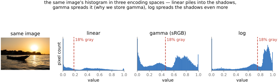
The trap is simple: the shape of a histogram depends entirely on the numerical space the values are stored in. The same image (the same physical scene, the same pixels of light) has a completely different histogram in linear light than in gamma-encoded (sRGB) values than in a log encoding. Nothing about the scene changed; only the ruler we used to measure each pixel did, and the histogram is a picture of that ruler as much as of the scene (Figure 8.7.3).
Uniform bins in linear light count equal differences in light. Uniform log bins count equal ratios; sRGB allocates more numerical range to shadows than linear encoding does. Its main power-law segment uses exponent $1/2.4$, with an offset and a linear toe. These different bins give different histogram shapes even for identical pixels.
For a normalized linear value of 0.18, sRGB gives about 0.46. A log code value cannot be specified without the log curve, scale, and offset. Always label the encoding and range of a histogram, including whether the quantity is a channel, linear luminance, or encoded luma.
8.7.3 A histogram is a sampled estimate⧉
A histogram counts the values in the finite image exactly, subject to the chosen bins. As an estimate of an underlying scene distribution, it also reflects sampling and quantization:
Binning. You chose a finite number of bins (256 is common for 8-bit data), and the bin width sets the resolution. Too few bins smears real structure together; too many leaves the counts noisy and gappy. The comb-like ridges you sometimes see are an artifact of the bin grid, not the scene.
Quantization. If the underlying values are themselves quantized (an 8-bit image has only 256 distinct levels) then the histogram inherits spikes and gaps: tall counts at the levels that exist and empty bins between them. This is especially severe after a stretch (levels or equalization), which spreads 256 input levels across a wider output range and leaves visible combing. Those gaps are an artifact of the quantization, not evidence of anything about the photograph. Read the overall shape (where the mass sits, whether it clips) and do not over-interpret the fine teeth.
8.7.4 Histogram equalization⧉
Now use it: the histogram can drive an automatic tone curve. The classic move is histogram equalization, and it rests on one clean idea. Recall the cumulative histogram, or cumulative distribution function (CDF), the running total of the histogram, swept from black to white, climbing monotonically from 0 to 1. Use that CDF as the tone curve itself:
That is the entire algorithm: build the image's CDF, then push every pixel value through it. Concretely, count the pixels into bins, sweep left to right accumulating a running total, normalize it to climb from 0 to 1, and use the result as a per-pixel look-up table:
# Finite scalar values in [0,1], nonempty image, B >= 2.
# Preserve a constant image: it has no contrast to redistribute.
if min(im) == max(im): return copy(im)
bin(v) = min(B-1, floor(B*v))
hist = zeros(B)
for v in im: hist[bin(v)] += 1
cdf = cumulative_sum(hist) / number_of_pixels(im)
for p in pixels(im): out[p] = cdf[bin(im[p])]
There are two ways to see why this works, one about ranks and one about slopes.
The CDF at a value $v$ is the fraction of pixels darker than $v$, so mapping each pixel through it replaces its value by its rank: a pixel brighter than 30% of the image goes to 0.3, one brighter than 90% goes to 0.9. The darkest tenth of the pixels therefore lands in $[0, 0.1]$, the next tenth in $[0.1, 0.2]$, and so on. Every tenth of the output range receives a tenth of the pixels, which is what a flat histogram means. The curve keeps the order of the pixels, since the CDF never decreases, and throws away everything else about their values: only how many pixels are darker matters.
The slope gives the same answer locally, and it is the version that explains what the curve does to contrast. The derivative of the CDF is the histogram itself, normalized: $\text{CDF}'(v)=h(v)$, the fraction of pixels per unit of value at $v$. A tone curve's slope is how much it stretches a small range of input values. A thin slice $[v, v+\Delta v]$ holds a fraction $h(v)\,\Delta v$ of the pixels and is stretched to an output range of width $h(v)\,\Delta v$, the same number. Output range is handed out in proportion to how many pixels need it. Where pixels crowd, the curve is steep and their small differences are stretched apart; where few pixels live, it is flat and spends almost nothing. For a continuous distribution the output density is exactly $h(v)/\text{CDF}'(v)=1$: uniform.
A small example makes the trade concrete. Suppose 80% of an image's pixels have values between 0.2 and 0.3, a dull, low-contrast scene, and the rest are spread from 0.3 to 1. The CDF climbs from 0 to 0.8 across $[0.2, 0.3]$, so that range of 0.1 is stretched to 0.8 of the output, a slope of 8: the crowded midtones gain eight times their contrast. The remaining 0.7 of the input range is squeezed into the last 0.2 of the output, a slope below 0.3, and loses contrast. Equalization spends contrast where the pixels are, which is the same budgeting argument that drives tone mapping of high-dynamic-range images (Chapter 18.2, Global tone mapping).
In Figure 8.7.4 a band of input levels is projected through the CDF onto an output interval as wide as its share of the pixels.
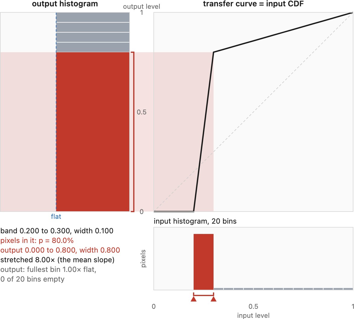
A finite image has ties: all pixels at one input value receive the same output, so a deterministic curve cannot split their count among several output bins. Equalization allocates more output range to crowded tones, but does not guarantee a flat discrete histogram or maximize every measure of contrast. In the worked example above with bins 0.05 wide, the two crowded bins become two spikes of 40% each, and only four of ten output slices receive any pixels: equalization stretches the range between crowded values, but cannot split a single value.
Once computed, the CDF is a point operation, conveniently stored in a LUT. Choosing that curve is image-dependent. There is a useful distinction from histogram shape: a strictly increasing encoding preserves ranks. For such an encoding $g$, $F_{g(L)}(g(L))=F_L(L)$. Ideal CDF equalization therefore gives the same output ranks before and after encoding. Finite bins, quantization, ties introduced by clipping, and the chosen output encoding can change the practical result.
Equalization has no model of subject matter or noise. A nearly uniform wall can occupy many pixels but a narrow range of values; equalization stretches that range and makes its noise conspicuous. Use it cautiously for photographic contrast.
Figure 8.7.5 applies the CDF to synthetic and real images, shows the histograms before and after, and follows one gray level through the curve.
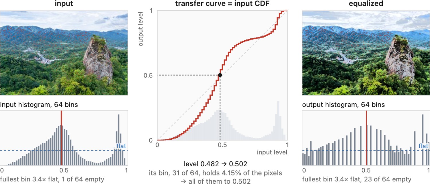
A narrow cluster in the input histogram makes the CDF rise steeply there. Applying that CDF as a tone curve spreads the cluster over a wider output range, increasing distinctions among those pixels. If the cluster was mostly noise in a smooth wall, the same operation increases the noise contrast. An image-wide histogram cannot tell the difference between useful texture and unwanted variation. This explains why a mechanically well-defined equalization can give an unattractive photograph, and why limiting the curve's slope or using another rendering criterion can help.
8.7.5 Histogram matching⧉
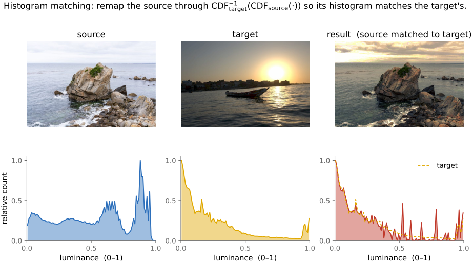
Equalization flattens to a uniform target. But why uniform? Histogram matching (also called histogram specification) generalizes the idea: reshape an image's histogram to match any target distribution you like (a chosen shape, or, more usefully, another image's histogram). You hand it a reference and it makes your image's tonal distribution look like the reference's.
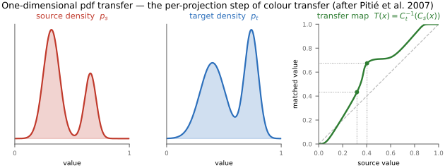
The recipe: compose two CDFs. First equalize the source, push it through its own cumulative distribution $\text{CDF}_\text{src}$, which (as we just saw) flattens it to a uniform spread. Then un-equalize through the target's inverse CDF, $\text{CDF}_\text{tgt}^{-1}$, which reshapes that uniform spread into the target's distribution. Composed into one curve:
For a discrete target, use the generalized inverse: the smallest target value whose CDF reaches the requested probability. Ties prevent an exact match in general. Splitting ties by position or randomness changes the operation from a curve of value alone.
Both pieces are one-dimensional, so their composition is one-dimensional too: matching is still a single point operation, a LUT applied per pixel (Figure 8.7.6). And equalization falls out as the special case where the target is uniform, so $\text{CDF}_\text{tgt}$ is the identity and the formula collapses back to $L_\text{out} = \text{CDF}_\text{src}(L_\text{in})$. Matching, equalization, and a hand-drawn levels curve are therefore one family: all of them one monotone curve on the value axis, differing only in how the curve is chosen.
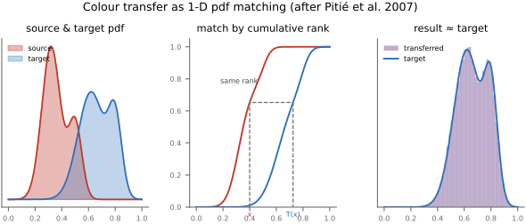
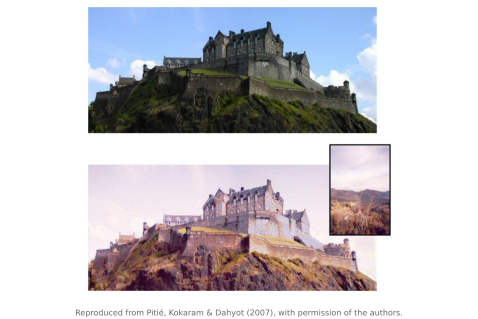
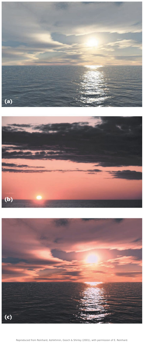
For color, independent RGB matching changes channel relationships and can shift hues. Reinhard et al. Reinhard et al. 2001 instead match channel means and standard deviations in $l\alpha\beta$, a space designed to reduce channel correlation. This reduces one source of interference; it does not guarantee preservation of hue. Pitié et al. Pitié et al. 2007 repeatedly match one-dimensional projections of the color distribution. This addresses joint color statistics, but is not a guarantee of a minimum-cost transport map or unchanged hues. Distribution matching alone also lacks the spatial information needed for general relighting; portrait methods such as Shu et al. 2017 (portrait lighting transfer) impose additional structure.
For a source channel $x$, moment matching uses
The subscripts denote source and target statistics. If $\sigma_s$ is zero, the source channel contains no variation to stretch; mapping it to $\mu_t$ is a reasonable fallback. A small denominator can amplify noise, so practical implementations limit the gain. The statistics are computed after conversion to $l\alpha\beta$, not directly on raw sensor values. Feature-statistic matching in neural style transfer Gatys et al. 2016 uses a related idea on learned features.
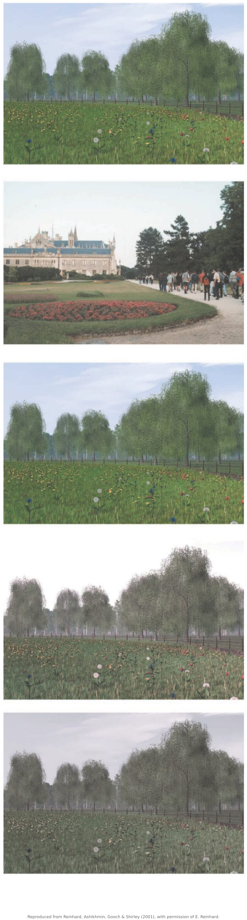
The textbook treatment of the one-dimensional case is Gonzalez & Woods Gonzalez & Woods, Digital Image Processing.
Histogram and color matching turn out to be a workhorse far beyond this chapter. The same "make this image's statistics look like that one's" move powers harmonization (making a pasted region's tones match its new background, see Chapter 19.1, Transparency and compositing), color grading and style transfer (imposing a reference look), and even texture synthesis (matching value statistics). It is one of those small ideas that keeps reappearing.
Two images can share every per-channel histogram and still contain different colors. For a two-pixel example, compare red plus cyan with yellow plus blue. In each case the red, green, and blue channels each contain one zero and one one, so their three marginal histograms agree. Their RGB triples do not. Independent channel matching has no information about which channel values occurred together. A joint color model retains that association, though it still does not describe where the colors occur or what objects they belong to. This is why matching color statistics alone cannot reproduce an arbitrary spatial lighting arrangement.
8.7.6 Constraining the slope: Ward's histogram-based tone mapping⧉
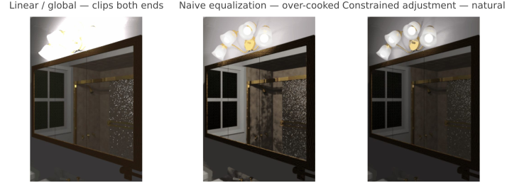
Ward Larson, Rushmeier, and Piatko Ward et al. 1997 constrain histogram adjustment using a model of visible contrast. The method works with brightness-related values and limits how much the mapping can increase contrast. It retains the histogram's adaptation to the image while reducing the excessive contrast of unconstrained equalization. The perceptual model is a design constraint, not a guarantee that every viewer will prefer the result.
The HDR comparison in Figure 8.7.12 shows linear scaling, unconstrained equalization, and constrained histogram adjustment. Figure 8.7.13 plots their transfer curves. Label both axes before interpreting a slope: a slope in log luminance expresses a change in relative contrast, unlike a slope in linear luminance. See Chapter 18.2, Global tone mapping for the display-range problem and Part 18, Tone mapping and display for a broader comparison.
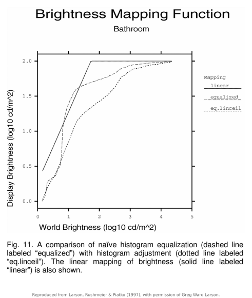
The link between the histogram and the constraint is the derivative of the mapping. In the continuous case, the derivative of the CDF is the probability density: densely populated values receive the steepest equalization curve. Limiting that slope restricts the contrast allocated to those crowded values. In log luminance, this controls how much nearby luminance ratios are expanded. The operator can still adapt its allocation to the image without letting pixel counts alone dictate arbitrarily strong local contrast.