8.6 Color beautification and preferred colors⧉
A photographer may prefer a bluer sky or warmer skin than a neutral rendering produces. Such preferences are appearance choices, not corrections to the measured color. A color look can implement them with hue-selective adjustments, but a pixel’s color alone does not tell us which object it belongs to.
Colorimetric accuracy and preferred reproduction are different objectives. Preferences depend on the viewer, subject, context, and intended style. Keep a neutral rendering available and evaluate selective changes across varied images and skin tones.
8.6.1 Accurate is not preferred⧉
Bartleson found systematic differences between remembered colors of familiar objects and their measured colors Bartleson 1960 (memory colors). Subsequent work studied preferred reproduction Bartleson & Bray 1962 (preferred reproduction). In Bartleson's measurements, remembered sky was bluer and more saturated than real sky, remembered grass greener, and remembered skin cleaner and more uniform than the measured skin; Bartleson and Bray found the best-liked reproductions pulled the same way. These results motivate memory-color adjustments, but do not establish one preferred hue or saturation for every person and image.
A cyanward sky adjustment is one possible style. A magenta-looking sky can also signal an incorrect white balance, profile, or gamut conversion. Check calibration before treating every color complaint as a preference problem.
We build that stage at the bottom of a complexity hierarchy, as a pure color point operation: the pixel's own hue, saturation, and value decide the entire move, and nothing about where the pixel sits or what object it belongs to enters yet. That restriction is what makes the stage simple, and, as the last two sections show, it is also what breaks it. Classifiers and masks come later, in the world of local adjustments; here, color is all we are allowed to look at.
The distinction matters when choosing an evaluation target. A colorimetric reproduction asks how closely the output represents a specified measurement under specified viewing conditions. A preference experiment asks which rendering viewers choose. Familiar objects add a remembered reference that need not match either the present scene or another viewer’s memory. A technically accurate result can therefore lose a preference comparison without the calibration being wrong.
8.6.2 More vivid, but bounded: the naturalness constraint⧉
Increasing saturation does not guarantee increasing preference. Naturalness and preference experiments examine where enhancement becomes objectionable Yendrikhovskij, Blommaert & de Ridder 1999 (naturalness constraint). In Yendrikhovskij and colleagues' results, preference first rises as colors move toward their remembered prototypes and then falls once saturation passes what looks natural, an inverted U whose peak sits a little above the natural saturation distribution. Their results depend on the stimuli and viewing conditions; they do not give a universal saturation ceiling.
Bound the controls and taper them smoothly. Test skin with varied complexions and lighting rather than assuming that a narrow orange target suits every face. A uniformity control removes color variation as well as an unwanted cast.
Preferred is also not a universal constant. It is a tuned, per-vendor, partly cultural choice (a Fujifilm film simulation and a muted cinema look disagree on purpose), and it is set by preference experiments, paired comparison and expert-retouched datasets like MIT-Adobe FiveK, not derived from first principles. There is no equation for "preferred blue"; there is a measurement.
8.6.3 Three corridors, quantitatively⧉
Concretely, the stage acts through three corridors, one each for sky, foliage, and skin, and leaves every other color untouched. A corridor is a soft bump over hue: a weight $w(h)$ that rises to one at a center hue $h^*$ and falls smoothly back to zero at a half-width $W$ on either side, so the move fades in and out instead of switching on at a boundary. Two more tapers guard the edges of color space: the weight ramps up with saturation over roughly $s \in [0, 0.12]$ and with value over $v \in [0, 0.10]$, so that neutral grays and black receive zero weight while near-neutral and near-black colors receive a reduced weight. We work in display-referred HSV, hue in degrees.
The three corridors, with the numbers the book's raw developer actually uses:
1/ Sky blues, centered at $h^* = 215°$ with a half-width of $55°$ (reaching from about $160°$ to $270°$). The hue control reaches $\pm 20°$; a cyanward adjustment is one possible setting. 2/ Vegetation greens, centered at $h^* = 100°$, half-width $50°$ ($50°$ to $150°$), and a hue range of $\pm 20°$. The usual move is away from yellow and slightly deeper. 3/ Skin oranges, centered at $h^* = 25°$, half-width $28°$. This is deliberately the tightest corridor and the smallest range, $\pm 10°$: skin is where errors offend most, so the default moves it least.
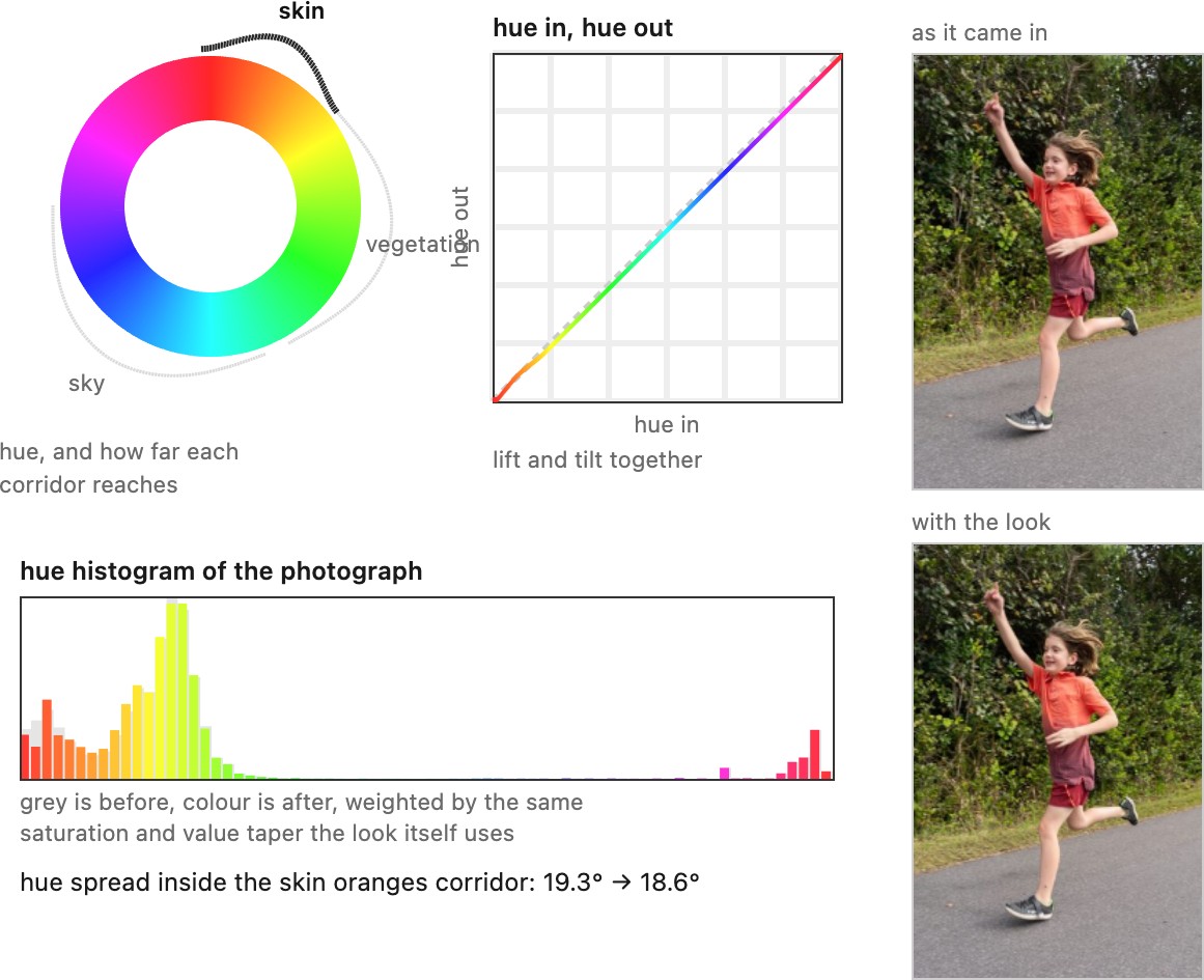
corridorApply; it is a copy, not shared code, so the figure and the Color Look panel of CompPhotoRoom have to be kept in step by hand. With the dress photograph, the scope switch gates each corridor's move by the probability that the pixel is sky, vegetation or person, as the raw developer's Color Look scope does, from the developer's own segmenter run once on the photo: the blue dress, which a pure color rule treats as sky, keeps its color when the moves are gated, and the three probability maps appear under the histogram.8.6.4 Two primitive moves: translate and contract⧉
Let $d$ be the shortest signed hue difference from the current hue to a chosen anchor, wrapped into $[-180^\circ,180^\circ)$. With a combined hue, saturation, and value weight $w$, combine translation and contraction as
At constant unit weight, translation adds $\Delta h$ and contraction alone has slope $1-k$. Hue must wrap across zero; ordinary subtraction gives the wrong direction near red.
The full tapered transform is not a rigid translation or a uniform contraction: the weight itself varies with hue, saturation, and value. Its derivative includes that variation, and overlapping adjustments can further change the mapping. Inspect the complete hue-in/hue-out curve for reversals or unexpectedly compressed ranges.
Contraction can reduce a selected hue spread, for example an unwanted cast variation across a portrait. Whether that is desirable depends on the image. Strong contraction can erase skin variation, makeup, or lighting cues. Preserve the original and make the effect adjustable.
For the untapered contraction alone, two nearby hues on the same side of the wrap boundary move closer by the factor 1-k. With 0<k<1 each travels partway toward the anchor without crossing it. Translation moves their mean without changing their separation. This is why shifting a cast and reducing hue variation are different controls: one changes the center of a distribution, the other its spread. The same distinction can be used for saturation, with suitable bounds.
8.6.5 The oldest shipped example: NTSC flesh-tone correction⧉
Analog television provides an earlier example of selective color handling. NTSC’s YIQ representation allocated different bandwidths to two chroma axes Wintringham 1951 (NTSC colorimetry). That perceptual bandwidth allocation and receiver flesh-tone correction are related historical ideas, but are not the same operation.
Some receivers used flesh-tone correction to pull a selected hue range toward a preferred reference when transmission errors shifted color. A digital hue curve or profile table can perform a similar contraction. Neither a television chroma axis nor a narrow hue corridor describes every human complexion and illumination.
Receiver makers then went further and shipped automatic tint, or flesh-tone, correctors: circuits that detected hues near the I axis and rotated them toward it. That is a hue contraction built in hardware, decades before any digital pipeline, and motivated by exactly the modern worry, since transmission phase errors shifted hues and an unwanted shift of facial color is especially conspicuous. Related digital mechanisms include profile lookup tables and a colorist’s hue-versus-hue curve with a deliberate flattening near a selected hue. They need not apply the same correction or target the same range. A hue selection alone is not a semantic skin detector.
8.6.6 The rung's documented failure⧉
A pure color point operation has one blind spot, and it is the whole reason the next rung exists: the stage cannot tell a blue car from the sky, or a wooden wall from a face. It sees only color, so anything whose color lands in a corridor gets that corridor's treatment, whether or not it is the object the corridor was meant for. A cyan car door is pushed toward sky-blue and gains "sky" saturation; a suntanned arm and a pine plank both answer to the skin move.
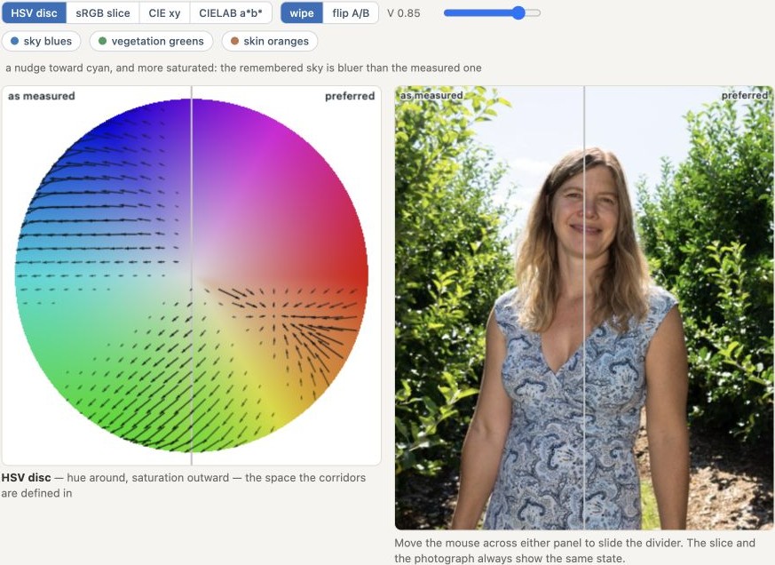
That is not a bug to be tuned away, it is the defining limit of operating on color alone. The fix is not a better corridor. It is a different kind of information: knowing what the pixel is, not only what color it has.
8.6.7 Semantic gating by object detection⧉
Let $\Delta_{\rm color}(p)$ be the color-only adjustment at pixel $p$. A semantic score $P(p)$ in $[0,1]$ gates it:
The detector supplies additional evidence about where the color adjustment belongs. A correct sky mask excludes a blue car; a mistaken mask still edits it.
The inspected raw-developer code uses a SegFormer-B0 model trained on ADE20K, with a 512×512 input and three aggregated 128×128 maps. They represent sky, vegetation, and person. The field named skin is a person map, not a skin detector: clothing and hair can receive its weight. Combining it with a hue corridor narrows the affected colors but does not turn it into semantic skin segmentation.
Low-resolution masks reduce inference cost but can miss fine boundaries. The application upsamples its semantic maps bilinearly, which softens their boundaries. Guided or joint-bilateral upsampling are possible alternatives for semantic masks; the application currently offers them for depth maps instead. They can align transitions with image edges while also copying the wrong edges. A larger network input can improve effective image-space detail despite a fixed output stride. Soft class scores make the effect gradual, but may be confidently wrong and are not automatically calibrated probabilities.
The classical detectors this replaces were the corridors with position added: sky is blue and near the top of the frame, skin is orange and inside a detected face. Those were chromaticity corridors plus hand-drawn spatial priors, the machinery of this chapter with a location term bolted on. The network swaps the hand-drawn priors for learned ones; the interface, a per-pixel weight in $[0,1]$, is unchanged.
The same maps pay a second dividend. They are exactly the masks behind semantic local adjustments, the "Select Sky" and "Select Subject" buttons in a modern editor: the mask is the weight map, and any slider can ride it. One mechanism serves two consumers, the automatic look and the user's own masked edits.
Keep these appearance choices in the editable rendering recipe. Preserve scene-linear data for later physical reconstruction, and state the working space of any processing performed after the color look.
Recap: big lessons of this chapter
Colorimetric accuracy and preferred reproduction are different objectives. Preferences depend on the viewer, subject, context, and intended style. Keep a neutral rendering available and evaluate selective changes across varied images and skin tones.