8.4 Beauty curves: the camera "look"⧉
A neutral raw development and a camera JPEG can look quite different even when both use correct color conversion. The JPEG may have deeper blacks, brighter midtones, and less abrupt highlights. These differences come from rendering choices, including tone curves and color adjustments. Radiometric calibration does not determine the preferred appearance.
Keep calibrated scene data available for operations that require it. A rendering transform chooses how that data appears on an output device. It can combine a tone curve, color adjustments, and gamut mapping; output encoding remains a separate specification.
8.4.1 Why scene-linear looks dull⧉
A scene’s range may exceed the display’s, and its lighting may not produce the contrast wanted in the photograph. A plain transfer encoding solves neither problem. However, linear data correctly exposed and encoded need not look dull: 0.18 linear already encodes to about 0.461 in sRGB. A missing tone curve is only one possible cause of a dark raw render; incorrect exposure normalization, black levels, or color calibration can also be responsible.
Tone mapping and a camera look overlap. A curve can both compress highlights and add midtone contrast, even for an ordinary photograph. Chapter 18.2, Global tone mapping discusses range compression; this chapter concentrates on choosing the baseline appearance. There is no universal one- or two-stop correction that every raw render needs. Why a pleasing rendering needs more midtone contrast than the scene had, and how much, has a largely perceptual answer, given in #Perceptual basis for beauty curves at the end of this chapter.
8.4.2 The shape of the curve⧉
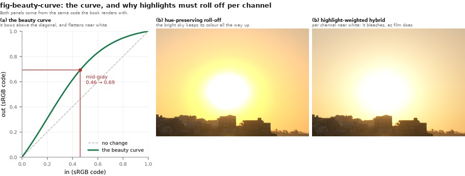
A tone curve specifies input and output units, a black behavior, a midtone response, and a highlight behavior (Figure 8.4.1). Monotone curves avoid tone reversals. Smooth slopes reduce abrupt contrast changes, but a continuous curve cannot prevent banding introduced by coarse output quantization. Parametric curves and interpolated tables are both useful.
A camera profile or photographer chooses the shape. Fitting raw/JPEG pairs can estimate a curve only after accounting for exposure, color conversion, and local processing; matching luminance histograms alone does not uniquely identify the camera pipeline. Evaluate a candidate on varied scenes rather than treating a fitted parameter set as a physical calibration.
A curve can be authored in scene-linear, log, or encoded coordinates. These choices give different parameter meanings and can represent the same composite mapping when converted correctly. State which one is used. In particular, sensor saturation normalized to 1 is not the same reference as diffuse scene white or display white.
Where does the exact shape come from? In a real camera or in Lightroom it is part of the camera profile (Adobe's "Adobe Standard"/"Adobe Color" DCP carries a baseline tone curve, on top of which sit a HueSatMap and a creative LookTable). For this book the shape is a handful of numbers rather than a table: an S about a pivot, with the strength of the S and the position of the pivot the two that matter, and a black point, a midtone lift and a shoulder available beside them. We began by fitting the curve the way you would expect, matching our render's luminance distribution to a Lightroom-developed JPG across a set of photographs, and obtained a visual match. What it taught us is that it had too many knobs. Several parameters can compensate for one another over the sampled range, so the fit could trade them against one another and the numbers it returned said less than they appeared to. Comparing the curve by eye across twenty-two photographs led to a simpler S-curve. This was a rendering choice, not a unique recovery of Lightroom’s processing.
The pivot illustrates why the units matter. Eighteen percent linear encodes to about 0.46 in sRGB, so 0.18 is not the corresponding encoded-domain pivot. There is a second distinction in a raw file: a normalized value of 1 often denotes sensor saturation. Exposure may leave substantial headroom above diffuse white for reflections and light sources. A pivot chosen relative to sensor saturation therefore need not coincide with a nominal middle-gray code value. Our low pivot was an appearance choice for the photographs being rendered, not a new definition of middle gray. Measured over our own photographs, the brightest one percent of the frame lands anywhere between 0.35 and 1.0 of the sensor's range, which puts the scene's own middle gray between code 0.28 and 0.46; the pivot chosen by eye sits near 0.20, below all of them.
8.4.3 Highlights: roll off to white, not to a color⧉
Scaling all three linear RGB channels by one factor preserves their ratios and chromaticity before clipping. This can keep bright colors too saturated for the intended look. Applying a curve separately to channels can desaturate some highlights but also shift hue; pure primary colors need not approach white. Highlight desaturation and gamut compression should therefore be explicit rendering choices, tested on skies, sunsets, and saturated lights.
8.4.4 Saturation, and the rest of the "look"⧉
A look may also adjust chroma selectively. Chapter 8.5, Color point operations distinguishes saturation controls from vibrance; Chapter 8.6, Color beautification and preferred colors discusses preference-driven adjustments. Keeping Oklab lightness and hue coordinates fixed while changing chroma is a useful construction, not a guarantee of exact perceived hue or lightness after gamut mapping. A skin-colored hue range also includes objects other than skin.
Our rendering experiment used Oklab chroma with a gain that decreased as colors became stronger, plus a reduction around orange-red hues to limit changes to faces. This is a hue-based precaution, not a face detector. HSV saturation alone is a poor measure of how colorful a pixel appears: scaling all RGB channels down preserves HSV saturation while making the color much darker. A chroma measure in a perceptual space allows lightness and gamut limits to enter the decision explicitly. The normalization still needs a definition, since the available chroma depends on hue and lightness. Stronger gains can make foliage and skies look implausible; compare them with skin and neutrals when tuning the look.
8.4.5 Vignetting and grain, added on purpose⧉
Two parts of a look are defects that photographers ask for by name. A lens darkens the corners of its frame, and film records an image in grains of silver halide rather than on a uniform grid. Both were things to correct, and both survive as deliberate effects.
Post-crop vignetting darkens toward the corners as a smooth function of radius from the center of the cropped frame, which is why editors offer it separately from the lens-profile correction that removes the optical vignetting of Part 22, Compound lenses, and aberration correction. The correction and the effect are the same operation with opposite sign, and an editor usually applies both: first flatten what the lens did, then darken what the photographer wants darkened. Applying it in scene-linear light changes saturation differently from applying it after the tone curve, so a look specifies where in the chain it belongs.
Grain is added noise with structure. Film grain is not white: the grains have a size, so the noise has a spatial correlation, and there are more of them in the midtones than in the extremes, so its strength varies with exposure. A convincing emulation therefore has a grain size, a per-tone strength, and usually a per-channel correlation, which is what separates it from the sensor noise of Chapter 2.8, Noise, signal-to-noise ratio and dynamic range that the pipeline spent its denoising budget removing. Adding grain after denoising is not an admission of defeat: a small amount of correlated noise hides the plastic look that aggressive denoising leaves, and it gives compression something to preserve rather than smooth away.
8.4.6 Our curve, in code⧉
Here is a small illustrative rendering transform, not a reproduction of a particular editor. It maps scene-linear luminance to display-linear luminance, scales RGB to match, then optionally desaturates bright values toward white. The final sRGB encoding is separate. The curve and highlight weight are appearance parameters.
# Input: nonnegative scene-linear RGB with Rec.709 primaries.
# T: chosen tone curve, linear luminance -> display-linear luminance in [0,1].
Y = dot(rgb, [0.2126, 0.7152, 0.0722])
Yout = T(Y)
if Y == 0:
    mapped = [Yout, Yout, Yout]
else:
    mapped = rgb * (Yout / Y)
h = chosen_highlight_desaturation_weight(Yout)  # bounded to [0,1]
mapped = (1-h) * mapped + h * [Yout, Yout, Yout]
mapped = gamut_map(mapped)                     # target display gamut
output = srgb_encode(mapped)
For a simple bounded curve, use $T(Y)=Y/(Y+a)$ with $a>0$. To map a positive input pivot p to output q, where $0<q<1$, choose $a=p(1-q)/q$. The output approaches white as Y grows. This curve is an example, not a full camera look. Negative working values need a defined treatment before this nonnegative-input version; blindly clipping them earlier can change color.
A lookup table is convenient when a photographer wants to edit the curve directly. The following three implementations use the same illustrative 17-point table and the same highlight blend. These are appearance choices, not a recovered camera profile. Here both the table input and output are explicitly linear-light values; encode the result afterward for display.
The table is sampled uniformly on [0,1]. We multiply the input by 16, find the two neighboring entries, and linearly interpolate. This example clamps outside that interval, so it deliberately clips scene headroom above 1. A production scene-referred curve can instead use a wider or logarithmic input axis.
import numpy as np

BEAUTY_LUT = np.array([0, .30, .42, .50, .57, .63, .68, .72, .765,
                      .80, .835, .865, .89, .915, .94, .97, 1.0])
LUMA = np.array([.2126, .7152, .0722])

def curve(value):
    t = np.clip(value, 0, 1) * 16
    i = np.minimum(t.astype(int), 15)
    f = t - i
    return BEAUTY_LUT[i] * (1-f) + BEAUTY_LUT[i+1] * f

def beauty(rgb, saturation=1.10):
    # Finite, nonnegative scene-linear RGB, final axis has three channels.
    rgb = np.asarray(rgb, dtype=float)
    Y = rgb @ LUMA
    t = np.clip((Y - .5) / .5, 0, 1)
    h = t*t*(3-2*t)
    scale = np.divide(curve(Y), Y, out=np.zeros_like(Y), where=Y > 0)
    mapped = rgb * scale[..., None] * (1-h[..., None]) + curve(rgb)*h[..., None]
    Ym = mapped @ LUMA
    s = 1 + (saturation-1)*(1-h)
    return np.clip(Ym[..., None] + s[..., None]*(mapped-Ym[..., None]), 0, 1)
#include <algorithm>
#include <array>

static constexpr float BEAUTY_LUT[17] = {
    0, .30f, .42f, .50f, .57f, .63f, .68f, .72f, .765f,
    .80f, .835f, .865f, .89f, .915f, .94f, .97f, 1};

float curve(float value) {
    float t = std::clamp(value, 0.0f, 1.0f) * 16;
    int i = std::min(int(t), 15);
    float f = t-i;
    return BEAUTY_LUT[i]*(1-f) + BEAUTY_LUT[i+1]*f;
}

std::array<float, 3> beauty(std::array<float, 3> rgb, float saturation=1.10f) {
    // One finite, nonnegative scene-linear RGB pixel.
    const std::array<float, 3> w = {.2126f, .7152f, .0722f};
    float Y = w[0]*rgb[0] + w[1]*rgb[1] + w[2]*rgb[2];
    float t = std::clamp((Y-.5f)/.5f, 0.0f, 1.0f);
    float h = t*t*(3-2*t), scale = Y > 0 ? curve(Y)/Y : 0;
    std::array<float, 3> mapped;
    for (int c=0; c<3; ++c)
        mapped[c] = rgb[c]*scale*(1-h) + curve(rgb[c])*h;
    float Ym = w[0]*mapped[0] + w[1]*mapped[1] + w[2]*mapped[2];
    float s = 1+(saturation-1)*(1-h);
    for (int c=0; c<3; ++c)
        mapped[c] = std::clamp(Ym+s*(mapped[c]-Ym), 0.0f, 1.0f);
    return mapped;
}
#include <Halide.h>
using namespace Halide;

Func beauty(Func input, Buffer<float> lut, float saturation=1.10f) {
    // lut has extent 17 and minimum 0; finite samples match BEAUTY_LUT.
    // input is finite, nonnegative scene-linear RGB with channels 0,1,2.
    Var x("x"), y("y"), c("c");
    auto curve = [&](Expr value) {
        Expr t = clamp(value, 0.0f, 1.0f)*16.0f;
        Expr i = clamp(cast<int>(t), 0, 15);
        Expr f = t-i;
        return lut(i)*(1-f) + lut(i+1)*f;
    };
    Expr Y = .2126f*input(x,y,0) + .7152f*input(x,y,1) + .0722f*input(x,y,2);
    Expr t = clamp((Y-.5f)/.5f, 0.0f, 1.0f);
    Expr h = t*t*(3-2*t);
    Expr safe_Y = select(Y > 0, Y, 1.0f);
    Expr scale = select(Y > 0, curve(Y)/safe_Y, 0.0f);
    Func mapped("mapped"), output("beauty");
    mapped(x,y,c) = input(x,y,c)*scale*(1-h) + curve(input(x,y,c))*h;
    Expr Ym = .2126f*mapped(x,y,0) + .7152f*mapped(x,y,1) + .0722f*mapped(x,y,2);
    Expr s = 1+(saturation-1)*(1-h);
    output(x,y,c) = clamp(Ym+s*(mapped(x,y,c)-Ym), 0.0f, 1.0f);
    return output;
}
The luminance-scaled branch preserves channel ratios before clipping. The per-channel branch follows the curve on each component; the blend gives it more influence at high input luminance. This can reduce highlight saturation, but does not force a saturated primary to become white. For that behavior, use the explicit neutral blend in the preceding pseudocode. The final channel clamp is a simple gamut treatment for the example and can change hue; inspect saturated patches as well as the gray ramp.
For a neutral input, all three channels remain equal. Black maps to black, white maps to white, and the last table interval includes its endpoint without an out-of-bounds access. These are useful tests before trying a photograph.
8.4.7 The discipline⧉
Keep a non-destructive rendering recipe and retain the source data. Operations that model scene light belong before irreversible rendering; appearance adjustments and some gradient-domain edits may deliberately operate afterward in a different space. “Apply last” means after the scene-dependent operations it would invalidate, not that no processing may follow a tone curve.
Calibration and appearance are separate decisions. Preserve the calibrated source and specify the rendering transform. A pleasing result need not preserve scene radiance ratios, but later code must not mistake those rendered values for the original measurement.
5,000 RAWs retouched by 5 experts; the standard learned-enhancement set. <https://data.csail.mit.edu/graphics/fivek>. See the Chapter 45.16, Datasets appendix.
Use the beauty-curve demo to compare luminance scaling with explicit highlight desaturation (Figure 8.4.2). Saturated lights need not become white; inspect the intended color, gamut mapping, and roll-off together.
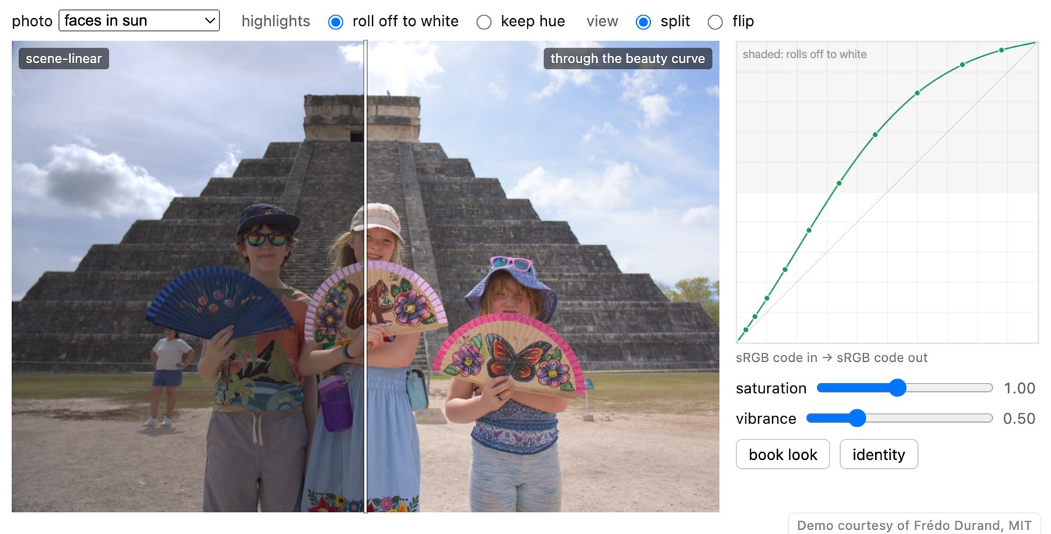
In Chapter 8.13, A raw developer in the browser this curve is the default Profile, and the menu beside it carries the rivals (Reinhard, Hable's filmic, a darktable-style sigmoid, the ACES fit), so the disagreement this chapter describes can be flipped through on one photograph. The Color Look stage is the color half of the same camera look.
8.4.8 Beauty curves in real ISPs⧉
Every pipeline in the ISP survey leaves scene-linear somewhere, and each applies a curve when it does. What separates them is whether the curve has a name. The raw editors give it a module you can open and switch off. Several embedded ISPs put it inside a table labeled "gamma", where it looks like a transfer function and is not only one. The values below were read from each project's source or shipped configuration on 2026-09-01 and can change with later versions.
darktable ships three generations of the answer and keeps all of them darktable. The oldest is the base curve: a spline of 6 to 20 nodes per camera model, contributed by users who shot raw and JPEG pairs and fitted them; the source describes it as a reverse-engineered conversion from scene-referred to display-referred. Its Nikon D750 preset runs $(0,0)$, $(0.018, 0.026)$, $(0.143, 0.370)$, $(0.330, 0.731)$ and on to $(1,1)$: a 14% tone comes out at 37%, a lift of about 1.4 stops. The newer modules replace the measured table with parameters. filmic rgb works in log exposure, places middle gray and the white and black relative to it, and joins a toe and a shoulder to a straight segment whose slope is the contrast control. sigmoid is the compact version: at zero skew it is $y = x^{c}/(x^{c} + K)$, with the contrast exponent $c$ defaulting to 1.5 and $K$ set so scene mid-gray lands on display mid-gray. It accepts scene-referred linear RGB and emits display-referred linear RGB, and all three run before the output profile in the pixelpipe, so the transfer encoding is a separate, later step (darktable sigmoid documentation).
RawTherapee applies no tone curve to a raw by default and then offers the hue question of the highlights section as a menu RawTherapee. Its curve modes answer what a curve should do to color. Standard applies the curve to each channel and accepts the hue shift (an orange drifts toward yellow under an S-curve). Weighted Standard blends per-channel variants to reduce that shift. Film-Like is the method of Adobe's DNG specification, a per-channel curve with the hue held constant in HSV. Saturation and Value Blending curves the pixel's mean and steers toward white as value rises. Perceptual scales chroma with the curve's local contrast (RawTherapee exposure documentation). ART, derived from RawTherapee, puts Adobe's camera-profile look elements (baseline exposure, tone curve, look table) on an early or late switch, and runs film-simulation HaldCLUTs in bounded gamma-2.2 RGB because those tables were authored there ART.
vkdt picks one parametric curve and exposes its parameters: filmcurv is a Weibull cumulative distribution, $y = 1 - e^{-(\ell x)^{k}}$, with light $\ell$ defaulting to 3 and contrast $k$ to 1.2, plus a choice of how to restore color after curving brightness. Its per-channel path ends with the saturation-preservation step of the DNG specification, the same recipe RawTherapee calls Film-Like. Its documented default raw chain includes denoising, highlight handling, demosaicking, crop, color conversion, the film curve and local processing, so a curve can define a rendering without being the last numerical operation.
In the embedded ISPs the curve loses its name. AMD Mini-ISP ends its compact black-level, gain, demosaic and color-matrix chain with the sRGB transfer function as a piecewise-linear table, and nothing follows it: the radiometrically correct, dull rendering this chapter opened with, shipped as a reference design. openISP builds its table as a plain square root and does its look afterward in the encoded domain: an 8-bit brightness and contrast stage, $Y \leftarrow Y + 10 + 0.3125\,(Y - 127)$, then a chroma gain. fast-openISP uses $x^{0.42}$ in its shipped Nikon configurations, followed by contrast-limited adaptive histogram equalization on luma. Neither power law is a beauty curve. The square root puts mid-gray below sRGB's, and $x^{0.42}$ lifts a half-percent shadow tone by more than a stop, which raises the black point rather than adding a look.
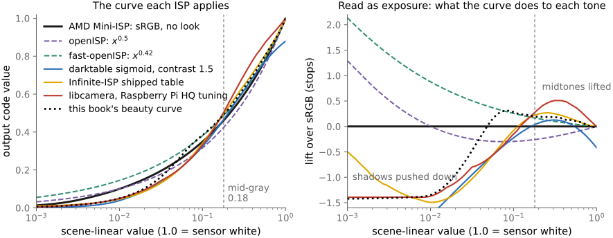
Infinite-ISP and libcamera are the two worth measuring, because each ships a hand-tuned table under the name gamma. Infinite-ISP's is 4,096 hand-supplied entries in its configuration file, followed by YCbCr conversion and display-oriented contrast, sharpening, saturation and denoising. The Raspberry Pi HQ camera's tuning file carries its contrast curve as 33 points, with the auto-exposure loop adding a histogram stretch at run time. Plotted against sRGB, both are S-curves: both put a 0.5% linear tone near code 0.025 where sRGB puts it at 0.061, and both lift mid-gray, to 0.495 and 0.504 against sRGB's 0.461.
On the same axes a third curve joins them (Figure 8.4.3). Our own beauty curve, recovered by fitting Lightroom's renderings of these photographs, puts the same shadow tone at 0.025 and mid-gray at 0.491. Three tables made by parties who were not copying one another, a raw editor's camera profile, an embedded-ISP vendor's table and a camera-module tuning, agree to within a few thousandths of a code value in the deep shadows and about a hundredth at mid-gray. Read as exposure, all three push a half-percent tone down by about 1.4 stops and lift the midtones by roughly a fifth of a stop. The two that disagree are the two whose table came from a power function.
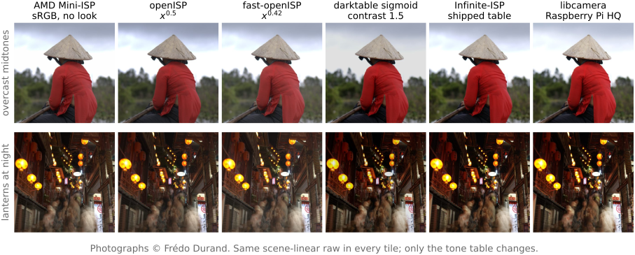
Applied to photographs, the tables differ the way the curves predict (Figure 8.4.4). On the overcast street, fast-openISP's $x^{0.42}$ turns the sky milky and lifts the shadows until nothing is black, while the S-shaped tables of Infinite-ISP and the Raspberry Pi tuning give the punchier midtones of a camera JPEG. The night street tests the shoulder. Its orange lanterns are saturated and partly past full scale, and a curve applied to each channel separately compresses the brightest channel first, so the lanterns' orange bleaches toward yellow and white as their cores approach the top of the curve. darktable's sigmoid desaturates the cores more softly, because it reaches display white only as its input grows without bound; this figure pins 1.0 at sensor white, whereas in darktable the exposure module normally places sensor white well above 1.0 first. Only the Mini-ISP rendering is the one this chapter calls correct, and it is the one nobody would publish. These comparisons isolate the scalar tables; they do not reproduce each application's complete rendering, which may differ in exposure normalization, working primaries, channel coupling and local processing.
Hiding the curve inside the gamma table has a cost: later stages cannot separate the look from the encoding. openISP's contrast stage, Infinite-ISP's luma enhancement and any stage that treats gamma as one more adjustment operate on values that already carry a look, and a stage that needs linear light back must invert a table that was never documented as invertible. Inverting a known monotone table recovers the preceding values up to quantization, but nothing lost to clipping or local edits. The raw editors pay for a named module and a separate output profile, and in exchange keep one place where the look is applied. Extracted tables are useful because they expose that distinction numerically: plot the stored mapping against the specified transfer encoding with both axes in the same units, and check exposure normalization and table placement before reading a difference as a camera look. The full pipeline context is in Chapter 8.12, Recap ISP, non-destructive editing.
8.4.9 Perceptual basis for beauty curves⧉
The S shape of a beauty curve is less a taste than a consequence of two constraints meeting. The midtones need a slope above one, for reasons below, and a scene's range is wider than the display's. A curve that is steeper than the diagonal through the middle and must still fit twelve stops into six has to bend at both ends. Once the midtone slope is fixed, the toe and the shoulder follow. The question is therefore where the extra midtone contrast comes from, and appearance science gives numbers for it.
Hunt separates the required overall gamma above one into four causes Hunt, The Reproduction of Color.
1/ Surround. An image seen against a dark or dim surround looks lower in contrast than the same image in an average surround, so its physical contrast must be raised to look right. Bartleson and Breneman measured this on complex images rather than isolated patches Bartleson & Breneman 1967 (surround), which is why it transfers to photographs. The customary system gammas are about 1.5 for a dark surround (cinema), 1.25 for a dim one (television at home) and 1.0 for an average one (a print viewed under the scene's own light). CIECAM02 encodes the same effect in its surround factor $c$, 0.69, 0.59 and 0.525 for average, dim and dark Moroney et al. 2002 (CIECAM02); Fairchild, Color Appearance Models.
2/ Absolute luminance, the Stevens effect: perceived contrast falls with adapting luminance Stevens & Stevens 1963 (Stevens effect), and a display is two or three orders of magnitude dimmer than a sunlit scene. BT.2100 writes this compensation down as a formula: the system gamma of its hybrid log-gamma mode depends on the display's peak luminance $L_W$ in cd/m², $\gamma = 1.2 + 0.42\log_{10}(L_W/1000)$ ITU-R BT.2100 (HDR-TV; ICtCp); ITU-R BT.2390. It is a rare case of a rendering intent specified in closed form rather than baked into a table (Chapter 18.10, HDR displays and display mapping).
3/ Flare, in the camera and in the viewing room, lifts the blacks and compresses shadow contrast physically; part of a curve's toe restores contrast that flare removed.
4/ Colorfulness, the Hunt effect: colors look more colorful at higher luminance Hunt 1952 (Hunt effect), so a dim reproduction with exact chromaticities looks less colorful than the scene, and restoring its appearance calls for a saturation increase.
Together, surround, luminance and flare put the midtone slope in the range of about 1.2 to 1.5 without any appeal to preference. What remains a matter of taste is narrower than it looks: where mid-gray lands, how the curve divides its compression between shadows and highlights, and how soft the knee is. The soft knee of the "filmic" look has no perceptual justification that we know of. Film's toe and shoulder came from the statistics of grains at low exposure and dye saturation at high exposure, and survived because people liked them.
Color is where preference takes over. The Hunt effect justifies some added saturation; consumer pipelines add more, and the excess goes to memory colors: greener grass, bluer sky, warmer skin Bartleson 1960 (memory colors); Bartleson & Bray 1962 (preferred reproduction). These preferences are stable enough across viewers to be predictable, but they are preference rather than restored appearance (Chapter 8.6, Color beautification and preferred colors). For skin the two pull apart, since the Hunt effect says to boost and preference says to protect, which is one reason vibrance controls leave skin hues alone (Chapter 8.5, Color point operations).
The film industry has made the split architectural. ACES separates an output transform, meant to carry the part that can be derived (range compression, surround and luminance compensation, hue behavior through the roll-off), from a look transform that carries the creative part ACES. Newer rendering transforms, AgX, OpenDRT, the ACES 2.0 output transforms and Khronos PBR Neutral, aim to make the derived half neutral, mostly by correcting the hue shifts of ACES 1.x, where saturated colors slid toward the primaries as they were compressed (AgX; OpenDRT; Khronos PBR Neutral). That history is the useful lesson: even the half meant to be objective carried unintended aesthetic choices, and separating the two proved harder than declaring the separation. Hunt and Pointer give a shorter treatment of the appearance effects Hunt & Pointer, Measuring Color.
Recap: big lessons of this chapter
Keep calibrated scene data available for operations that require it. A rendering transform chooses how that data appears on an output device. It can combine a tone curve, color adjustments, and gamut mapping; output encoding remains a separate specification.
Calibration and appearance are separate decisions. Preserve the calibrated source and specify the rendering transform. A pleasing result need not preserve scene radiance ratios, but later code must not mistake those rendered values for the original measurement.