8.1 Image representation⧉
PS1 builds the image class, point operations, and color (YUV, gamma, white balance). → Chapter 1.5, Problem sets (appendix).
The basics of representing images digitally are simple enough to make computational photography easy and fun for beginners: just two-dimensional arrays of red, green, and blue values. However, details matter, and you will save yourself a lot of trouble by paying attention to how exactly images encode information.
8.1.1 An image is an array⧉
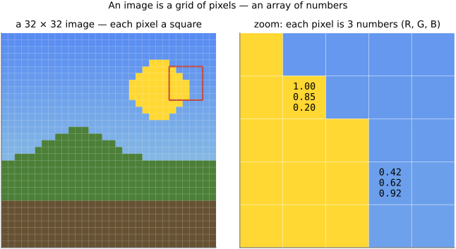
A color image is stored as a grid of channel values, commonly red, green, and blue (Figure 8.1.1). These are samples or measurements; drawing enlarged pixels as squares is a display convention, not a complete model of sensor integration.
More formally, an image is a function defined over a 2-D domain, the grid of integer positions $(x, y)$, whose values live in a range, here the space of colors. We store that function as a three-dimensional array of size $\text{height} \times \text{width} \times \text{channels}$ and write $I(x, y, c)$ for the value at column $x$, row $y$, channel $c$. A grayscale image has a single channel, and we drop the index and write $I(x, y)$.
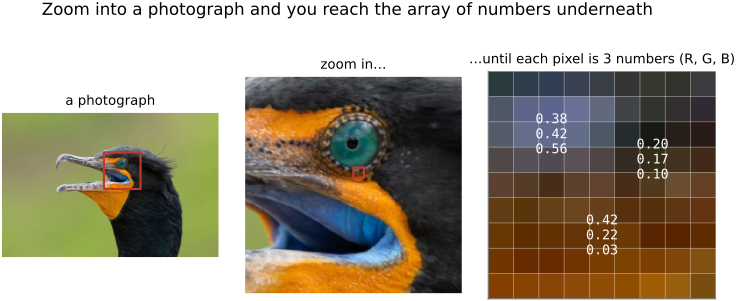
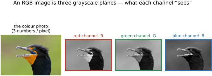
Usually a pixel carries exactly three channels, but nothing forces that. Some images add a fourth (for transparency, which we return to under alpha below) and scientific hyperspectral images keep dozens or hundreds of narrow wavelength bands instead of three broad ones. One very practical trap follows from this freedom, and it bites beginners constantly: a Portable Network Graphics (PNG) file may carry an alpha channel, so a file you assume is three-channel RGB hands you four channels instead. If the rest of your code expects three, every pixel downstream is misread. The fix is trivial once you know to look (check the channel count on load), but the symptom (colors scrambled, code not crashing) is hard to diagnose if you do not.
We use float32 for working images. Zero and one serve as black and reference white in normalized examples, but intermediate values may lie outside that interval. Changing an integer array to float changes its numeric representation; it does not decode its transfer function or identify its color space.
8.1.2 Float vs 8-bit vs more bits⧉
Use floating point for intermediate arithmetic. It provides more precision and headroom than 8-bit storage, but still rounds and can overflow. In normalized examples, 0 denotes black and 1 a chosen white level. Values above 1 can retain highlights; negative values can arise from noise after black subtraction, color transforms, or filters. Clip only where the next operation or output representation requires it.
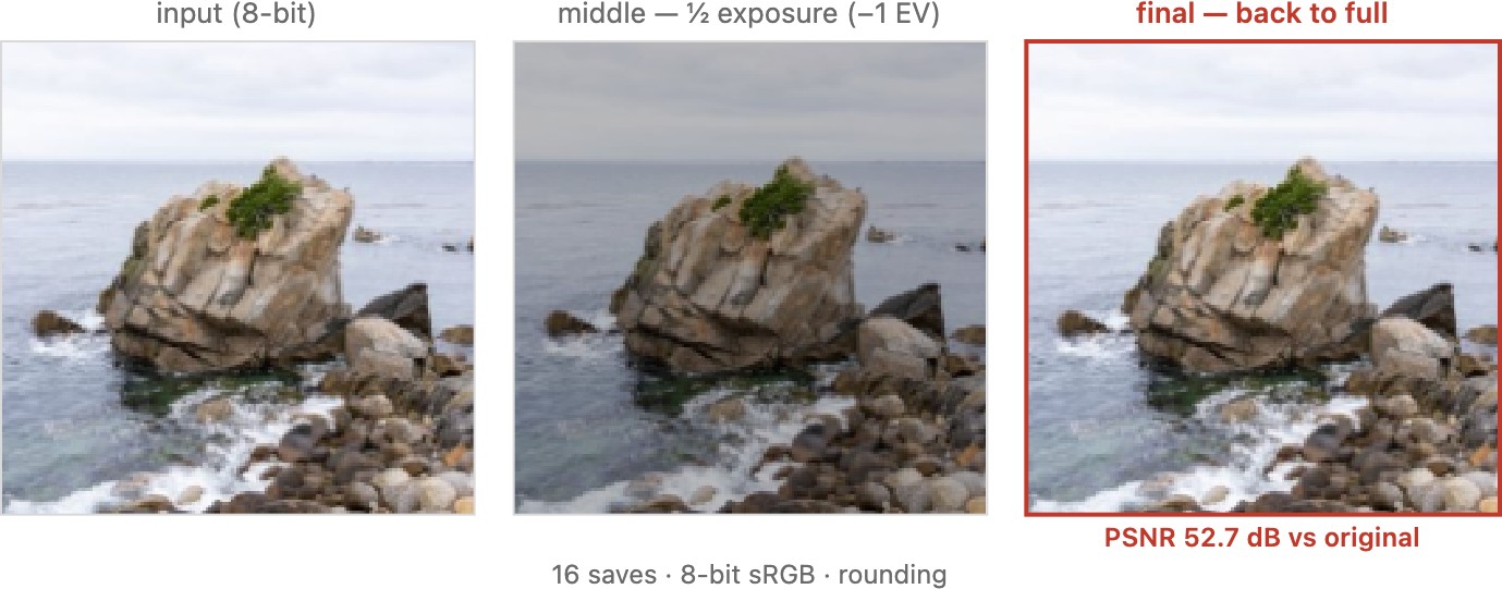
Repeated exposure changes followed by quantization are a stress test, not a model of every edit. The result depends on the step size, encoding, rounding, and clipping. More iterations need not monotonically worsen the image: sufficiently small changes can round back to the same codes. Gamma encoding allocates finer linear-light steps to shadows, but there is no universal equivalence between 8 encoded bits and a fixed number of linear bits.
💡 L2.47: when the quantization step is small relative to sensor noise, additional capture bits add little information. Coarse quantization, strong edits, and smooth synthetic gradients can still reveal banding. See Chapter 2.8, Noise, signal-to-noise ratio and dynamic range.
8.1.3 Stochastic quantization and dithering⧉
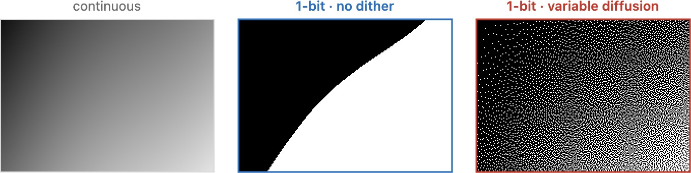
Dither replaces visible quantization structure with noise. Independent stochastic rounding produces approximately white noise; error diffusion shapes the error spatially and can leave patterns. Dither preserves an average under stated assumptions, not every pixel or every local region.
Stochastic rounding chooses between adjacent levels. For an input $v$ between $q_0$ and $q_1$, set $p=(v-q_0)/(q_1-q_0)$ and choose $q_1$ with probability $p$, otherwise $q_0$. Then $\mathbb E[q]=v$. This unbiasedness assumes no clipping and is expressed in the units used to define the levels. Independent decisions introduce noise with variance $p(1-p)(q_1-q_0)^2$ Gupta et al. 2015 (stochastic rounding).
Error diffusion passes each quantization residual to unprocessed neighbors. Floyd–Steinberg distributes it using weights $7/16,3/16,5/16,1/16$ in a raster scan Floyd & Steinberg 1976. Ostromoukhov varies the coefficients with intensity Ostromoukhov 2001. These methods shape the error rather than making it vanish, and can produce directional or periodic patterns.
To preserve average emitted light, use the actual linear-light values of the available output levels. For gamma-encoded levels, decode the two neighboring codes before calculating the rounding probability or residual. Simply dithering uniformly in code space preserves average code value, not average light. Boundary error loss and clipping can also bias error diffusion.
Capture precision and editing precision serve different purposes. Raw files often retain finer quantization and more highlight information than a rendered 8-bit image, but additional bits cannot recover a saturated photosite. A highlight clipped only by the rendering may remain available in raw. Sixteen-bit integers offer fine uniform steps over a fixed range; half floats offer a wider range with less significand precision. Choose the representation for the arithmetic and range, rather than treating all 16-bit formats as equivalent.
A float stores a number in binary scientific notation: sign × mantissa × 2^exponent. The exponent slides the binary point, so the same ~24 mantissa bits of a 32-bit float deliver the same relative precision whether the value is $0.001$ or $1000$. A few consequences matter for images:
- Precision is relative: fine near $0$, coarser for large values. That is a good match for linear radiance and high dynamic range (HDR) imaging, where you care about ratios, and roughly for how we perceive light (Weber's law).
- Intermediate headroom. Floating point can retain values above reference white and below zero. Individual operations may still clamp or require bounded inputs; document those boundaries.
- $0.1$ is not exact in binary, and adding numbers of very different magnitude loses the low bits (a long running sum of tiny values can drift). Usually negligible for images; occasionally not.
infandNaN(0/0,logof a negative,0 × inf) propagate and silently poison an image: one bad pixel can spread on the next blur. A classic bug; check for them when something goes mysteriously blank.float32is the working default.float16/ half halves memory (used in machine learning and some HDR pipelines) at the cost of precision;float64is rarely worth it for images.- Keep fine data centered near zero. Because precision is relative to magnitude, fine detail riding on a large offset (values clustered in a tight band around a big number, far from the origin) loses its low bits. The canonical illustration is Matt Pharr's note on why renderers work in camera space, not world space: pharr.org/matt/blog/2018/03/02/rendering-in-camera-space. Read it if your high-resolution data is not centered around zero.
Error diffusion gives the rounding a memory. If one pixel is rounded upward, its positive quantization error is subtracted from later inputs so that neighboring pixels can compensate. The resulting pattern trades spatial texture for a better local average. The average being preserved must be specified: averaging linear-light samples predicts emitted light, while averaging encoded samples preserves a different quantity. This matters for a one-bit projector or mask as well as for a displayed photograph. A locally correct average does not make the pattern invisible; viewing scale and the spatial distribution of error still matter.
For a value 70% of the way between two available levels, stochastic rounding chooses the upper level 70% of the time. Across many independently rounded pixels, the average approaches the desired value even though each individual pixel is quantized. At a viewing scale that blends the dots, this can replace a visible band with a textured tone. The same idea applies to a binary light mask or a projector with few available intensities: the spatial mixture approximates an intermediate response.
8.1.4 How the array sits in memory⧉
The array is two- or three-dimensional, but computer memory is one long line of numbered addresses. Something has to decide how the grid gets flattened into that line, and there is no single right answer. Different ecosystems made different choices, which matters the instant you pass an image between them.
The examples use packed planar C++ storage and HWC Python arrays. In contiguous planar storage, the element offset is $cWH+yW+x$; in contiguous interleaved storage, it is $(yW+x)C+c$ (Figure 8.1.6). A NumPy array can have other strides after slicing or transposition, and tensor dimension order does not uniquely determine physical memory layout. Query shape, strides, and contiguity at library boundaries. Row strides are $W$ elements per planar channel or $WC$ elements for interleaved RGB, before padding; byte strides also include element size.
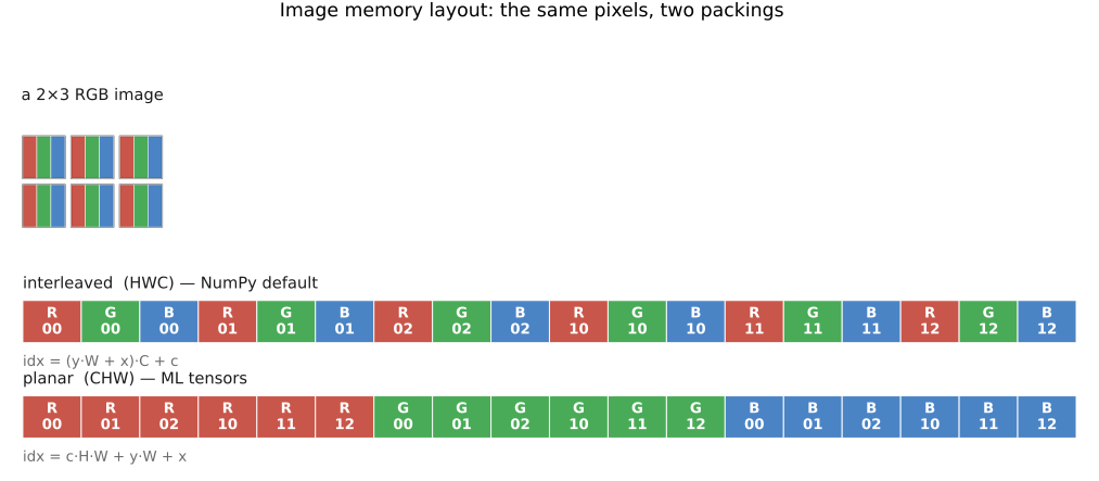
R G B R G B … row by row; pixel $(x, y, c)$ is at offset $(y\cdot W + x)\cdot C + c$. Planar (CHW): all of the red channel, then all of green, then all of blue, three contiguous planes; pixel $(x, y, c)$ is at offset $c\cdot W\cdot H + y\cdot W + x$. Same numbers, same picture; only the walk order through memory differs.The second decision is the order within a pixel. Most of the world, and this book, store the channels as red, green, blue (RGB), but a few libraries, OpenCV being the notorious one, use BGR. Mix the two and red and blue swap silently: skies turn orange, skin turns blue, and nothing throws an error. So always know which order your data is in.
Why care about any of this for everyday code? Mostly you should not. The mental model is just "a grid of pixels," and the accessor we build below hides the packing entirely. Two situations force you to think about it: performance (a loop that strides through memory in contiguous order runs far faster than one that hops around, so the right layout for an algorithm matters when speed does), and interoperability (handing an image to a library that expects a different layout means rearranging the array first). Outside those, the packing is an implementation detail.
Walking contiguous elements usually makes better use of cache lines and vector instructions. For packed HWC data, scalar loops run y, then x, then c; for planar CHW, c, then y, then x. A kernel that processes one whole pixel at once can hide the channel loop. Tiling, vectorization, compiler transformations, and hardware affect the best schedule; measure the implementation (Figure 8.1.7).
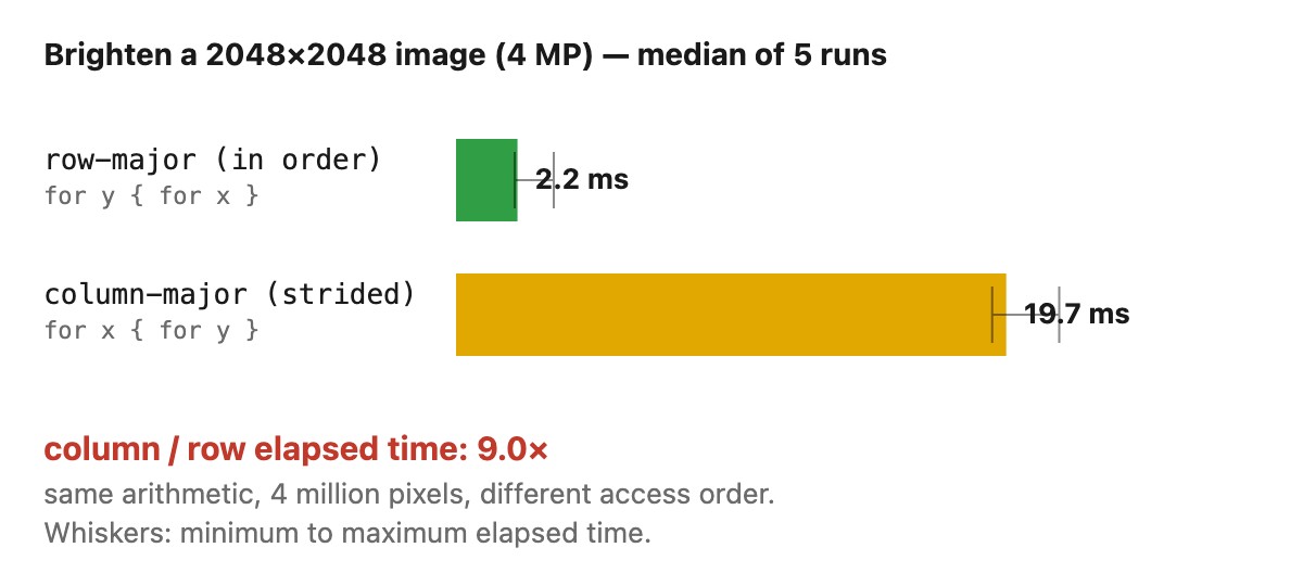
for y { for x } and the cache-hostile for x { for y }, warms up the JIT, then times several passes of each and reports the medians with their min–max spread. The arithmetic and the pixel count are identical; only the memory access order differs, yet the column-major walk typically runs several times slower on the very machine you are reading this on. Interactive: press Run to re-measure, and change the image size; watch the column-major bar stay several times longer than the row-major one, with tight whiskers showing the measurement is stable.Planar storage makes same-channel values contiguous. Interleaving keeps all channels of each pixel together, which can help operations that use them jointly. Vector implementations can handle either layout. Conversion costs and the whole pipeline matter more than declaring one layout universally faster.
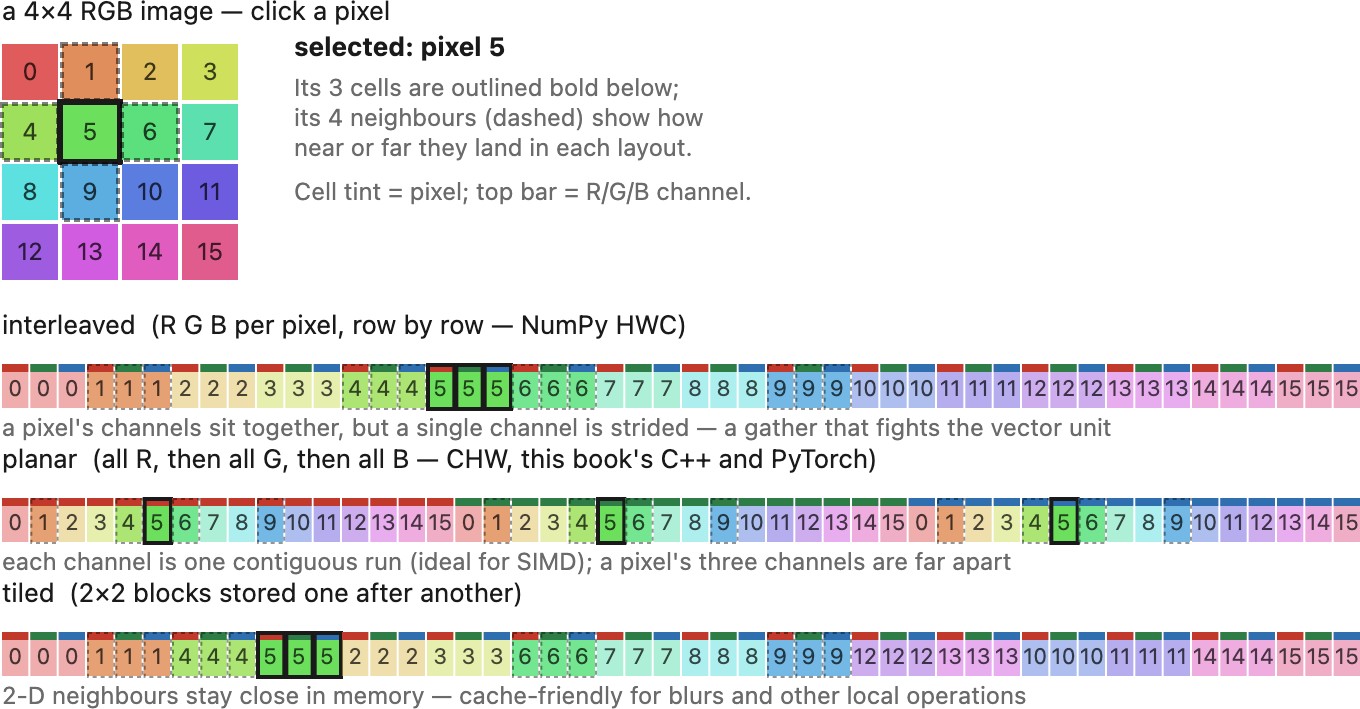
R G B together, row by row), planar (all the reds, then the greens, then the blues), and tiled (small 2×2 blocks laid one after another). To work on one channel, planar storage offers it as one contiguous run, the access a vector unit wants, while interleaving scatters it across every third cell. Tiled storage keeps a pixel's 2-D neighbors close together, which is what a local operation like a blur wants; no layout wins outright, you pick the one your access pattern rewards. Interactive: click a pixel to highlight its cells and its four neighbors across all three layouts, and flip the layout to watch the access pattern change.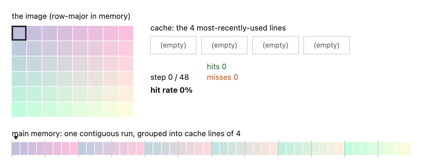
for y { for x } walks memory in order, so each miss loads a line that then serves the next several reads as hits; for x { for y } jumps a full row's stride every step, to a fresh line that is evicted before the loop returns, so almost every read misses. Same pixels, same arithmetic, very different hit rate. (A teaching model, real caches are larger and set-associative, but the locality effect is exactly this.) Interactive: play or single-step, and flip the loop order to watch the hit rate collapse.Prefer traversal that reuses nearby stored values. For scalar loops over packed HWC, use y, x, c order; for packed CHW, use c, y, x. Actual strides, tiling, and vectorized kernels can change the best schedule. Measure before changing the representation.
This book carries a concrete, working C++ image data structure; seeing it once makes the planar arithmetic above concrete. It is deliberately minimal: three integers for the shape, and a single flat buffer of floats in planar order:
struct Image {
    int width, height, channels;
    std::vector<float> data;        // planar: c*width*height + y*width + x

    Image(int w, int h, int c)
        : width(w), height(h), channels(c),
          data(static_cast<size_t>(w) * h * c, 0.0f) {}

    // The accessor: hides the index arithmetic, so the rest of the
    // code can think in plain (x, y, c).
    float& operator()(int x, int y, int c) {
        return data[static_cast<size_t>(c) * width * height + static_cast<size_t>(y) * width + x];
    }
};
This minimal accessor assumes validated nonnegative dimensions, a checked allocation-size product, and in-range indices. Use a sufficiently wide unsigned type for offset multiplication. A production image class also needs const access and explicit boundary reads; an unchecked mutable reference cannot implement zero padding safely. In Python, the book uses arr[y, x, c].
The accessor makes the storage choice concrete without spreading it through the rest of the program. A call such as img(x,y,0)=1.0f looks like indexing a three-dimensional image, while the function computes one offset into the flat buffer. Changing packing later requires changing this mapping and the code at library boundaries, rather than every mathematical expression. Read access beyond an image edge should be a separate policy from obtaining a mutable reference to a stored pixel.
The loop-order effect comes from reuse of fetched data. A cache line brings several neighboring values into the processor together. Traversing a packed row uses those values before moving on; jumping one full row per inner iteration can touch many cache lines while using only one value from each. A different schedule may recover that reuse through tiling or vectorization, which is why the benchmark measures the implemented loop rather than proving a universal ordering rule.
8.1.5 Pixel coordinate conventions⧉
Before we trust ourselves to index an image, two small geometric conventions have to be nailed down, because both are silent traps and both differ between tools.
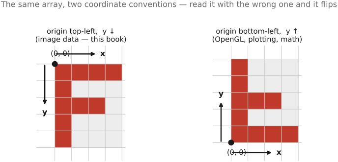
The first is where the origin sits. We place $(0, 0)$ at the top-left pixel, with $x$ increasing to the right and $y$ increasing downward: the order in which image data is scanned and stored, and the convention most imaging code (and our own camera frame) uses. The catch: a few systems (classic OpenGL textures, and much plotting and math software) put the origin at the bottom-left, with $y$ increasing upward, as on a graph. Hand an image from one world to the other without flipping it and the picture comes out upside down (Figure 8.1.10). Nothing crashes; it merely looks wrong, which is the worst kind of bug to chase.
We assign integer coordinates to pixel centers. A displayed pixel cell at $(0,0)$ spans $[-0.5,0.5)$ along each axis, and the image footprint spans $[-0.5,W-0.5)\times[-0.5,H-0.5)$. This geometric cell convention does not assert a box-shaped sensor response. APIs that place integer coordinates at cell corners differ by half a pixel.
That half-pixel sounds pedantic, and for a point operation it is: a curve applied to every pixel never asks where a pixel is. But the moment you resample or warp (scale up, rotate, correct lens distortion) you are evaluating the image at non-integer positions, and a consistent half-pixel error shifts the whole result by half a pixel, blurs it, or makes a "round trip" (shrink then enlarge) fail to land back where it started. It is one of the most common bugs in resampling code precisely because it never raises an error. We fix the convention now (integer = center) and return to it in full at resampling and warping, where it earns its own discussion of "where-from vs. where-to" addressing.
Keep two facts straight and most coordinate bugs evaporate: the origin is top-left, $y$ down, and an integer coordinate names a pixel's center, not its corner. Both are conventions, not laws: other tools choose differently, so check before you trust.
8.1.6 Alpha and extra channels⧉
So far each pixel has held three numbers, but nothing requires exactly three. The common fourth channel is alpha: a per-pixel opacity (or coverage) value, giving RGBA. Alpha carries one classic pitfall, premultiplied vs straight (whether the RGB values have already been scaled by the alpha), but we do not need it until Chapter 19.1, Transparency and compositing, which treats it in full. The heads-up for now is the narrow, very common one from the array section: load a PNG expecting three channels and you may get four, so check the channel count on load.
Beyond alpha, the array simply gains channels as the task demands. A depth (or Z) channel records distance per pixel; a matte marks out a region; hyperspectral imaging keeps many narrow wavelength bands instead of three broad ones (recall from the light chapter that "color," upstream of the camera, is really a full spectrum, hyperspectral keeps more of it). None of the machinery changes; there are just more numbers per pixel.
8.1.7 Video and more dimensions⧉
Nothing forces us to stop at a flat grid, either. A video is just an image sequence with one extra axis, time: $H \times W \times C \times T$. Most operations we write for a single frame generalize directly (run them frame by frame) and only the operations that couple frames (motion estimation, temporal denoising) need anything new, which we save for the motion and video material.
The same move works in other directions. Volumetric imaging stacks 2-D slices into a 3-D block: medical computed tomography (CT) and magnetic resonance imaging (MRI) produce an $H \times W \times D$ volume. A light field adds two angular axes to the two spatial ones (a 4-D record of rays, not just pixels); a spectral cube adds wavelength. In every case it is the same array machinery with more axes. We write this book for 2-D images and point out where adding a dimension is all it takes.
8.1.8 Pixel lookups and boundaries⧉
Almost every operation in the coming chapters reaches for a pixel's neighbors, which forces an unavoidable question: what is $I(x, y)$ when $(x, y)$ lands outside the image? We cannot dodge it, because blurs, gradients, resampling, and warps all ask for out-of-bounds pixels right at the border, where there are no neighbors on one side. Reading past the array is, at best, garbage and, at worst, a crash, so the first discipline is defensive: route every pixel read through a single accessor function, a small get(x, y, c), so that out-of-bounds access is decided in exactly one place rather than re-improvised (and re-broken) in every loop. As a bonus, that one function is also where the memory layout, the channel order, and the coordinate convention live, so the rest of the code can think in plain $(x, y, c)$ and forget every packing decision above. It is the natural home for one more safety check, too: asserting that an index lies in $[0, \text{size})$ inside that single function turns a distant, hard-to-trace crash into an immediate, localized error (we develop this habit in the debugging chapter).
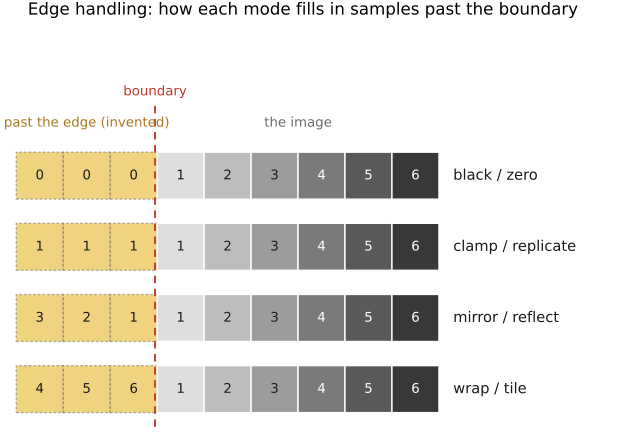
The accessor then has to decide what a pixel past the boundary means. There are four standard policies (Figure 8.1.11):
- black / zero: treat everything outside as $0$. Simple, but it darkens edges, since you are averaging in black that is not really there.
- clamp / replicate: repeat the nearest edge pixel outward. A reasonable, neutral default for many operations.
- mirror / reflect: fold the image back across its boundary, so the neighborhood just past the edge mirrors the one just inside. This avoids both the artificial darkening of zero and the streaking of clamp, and is the usual safe default for filtering.
- wrap / tile: treat the image as periodic, the left edge adjacent to the right. Rarely what you want visually, but it is exactly the assumption the Fourier transform makes, so it returns when we get there.
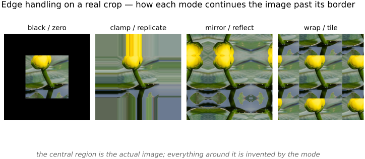
On a real photograph the four policies look like Figure 8.1.12: the same crop, continued past its border each way, surrounded by a dark frame, streaked outward, folded back on itself, or wrapped around from the opposite edge.
The boundary rule changes filtering and resampling near the border. We use reflection for these examples, stating whether the edge sample is repeated: libraries distinguish whole-sample and half-sample reflection. Neither reconstructs unseen content. For inverse problems, the adjoint must include the selected extension rule; see Chapter 6.9, Efficient linear solvers.
8.1.9 Three kinds of operation⧉
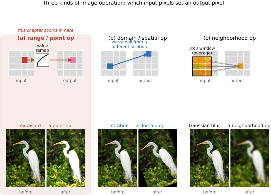
The domain/range split we just drew also sorts everything we will do to an image into three families, each the basis of one of the next several chapters (Figure 8.1.13):
- point operations touch the range only: a pixel's new value depends solely on its old value, the same rule applied everywhere (brightness, contrast, tone curves, gamma);
- domain operations change spatial coordinates; interpolation may also change values: each output pixel pulls its value from a different input location (translation, rotation, resizing, lens correction);
- neighborhood operations compute each pixel from a window of its neighbors (blur, sharpen, edge detection).
This is a preview; each family gets its own development later (point operations come first). But the taxonomy already earns its keep, because it predicts cost: a point operation reads each pixel once, while a neighborhood operation reads many input pixels per output pixel. We will flag which family every new tool belongs to as we go.
Recap: big lessons of this chapter
Dither replaces visible quantization structure with noise. Independent stochastic rounding produces approximately white noise; error diffusion shapes the error spatially and can leave patterns. Dither preserves an average under stated assumptions, not every pixel or every local region.
Prefer traversal that reuses nearby stored values. For scalar loops over packed HWC, use y, x, c order; for packed CHW, use c, y, x. Actual strides, tiling, and vectorized kernels can change the best schedule. Measure before changing the representation.