7.6 Information theory⧉
Information theory quantifies uncertainty, the dependence between measurements and scenes, and the cost of representing images. These quantities become useful only after specifying a source distribution, a noise model, or a distortion measure. They do not assign a universal number of “useful bits” to a photograph.
For practitioners, the most direct applications are compression, measurement design, and some estimation objectives. The distinction to keep clear is between a bound under a model and the performance of an actual camera or codec.
The historical survey separates two questions that are often merged. Is an information quantity actually the objective or bound being used, as in coding and some optical-system analyses, or is “information” only an informal description of lost detail? The distinction matters because an entropy, capacity or rate–distortion calculation earns its interpretation from its assumptions. Invoking the vocabulary alone does not supply that calculation.
7.6.1 The basics, at a high level⧉
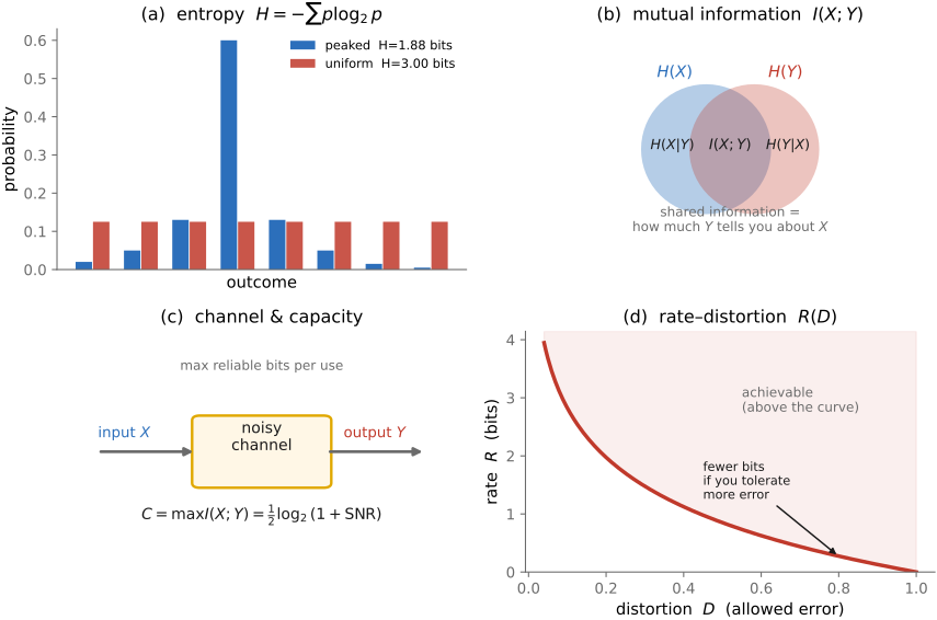
The basic quantities describe different questions [@shannon-1948; @cover-thomas-it] (Figure 7.6.1).
For a discrete random variable, entropy is
It bounds the average lossless description length under the source model. A uniform distribution on a fixed finite alphabet has maximal entropy per independent symbol. Dependencies between symbols can still make a sequence compressible. A pixel histogram therefore does not measure all the information in an image: shuffling pixels leaves histogram entropy unchanged while destroying spatial predictability.
Conditional entropy $H(X\mid Y)$ measures the uncertainty remaining after observing $Y$. Mutual information is $I(X;Y)=H(X)-H(X\mid Y)$. For discrete distributions,
is the extra ideal coding cost of using $q$ in place of $p$. It is nonnegative and asymmetric, and infinite if $q$ assigns zero probability to an outcome with positive $p$.
Channel capacity maximizes mutual information over the allowed input distributions. For a real scalar channel $Y=X+N$ with independent Gaussian noise of variance $\sigma^2$ and average input power at most $P$, a Gaussian input achieves
Rate–distortion $R(D)$ instead asks for the minimum rate needed to represent a specified source with expected distortion at most $D$. The answer depends on the chosen distortion measure.
These definitions use a probability model. For continuous variables, differential entropy depends on units and is not directly a file size; quantization must be specified before interpreting it as a number of stored bits.
7.6.2 Compression: the clearest application⧉
A codec spends bits on an approximate representation, balancing size against an application-dependent reconstruction error.
The theoretical rate–distortion function bounds achievable compression under a source model. A measured codec curve generally lies above that minimum rate. Huffman coding approaches the entropy with a possible per-symbol overhead; arithmetic and range coding can amortize overhead over long sequences, subject to model accuracy and implementation limits. Transform coding, such as JPEG’s DCT Wallace 1991, concentrates energy and reduces dependencies before quantization and entropy coding. The transform alone does not reduce the number of represented degrees of freedom.
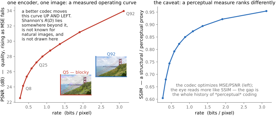
Rate–distortion theory permits perceptually motivated distortion measures; it does not require MSE. The difficulty is choosing a measure that matches the intended viewing conditions and task. JPEG’s quantization choices already include perceptual considerations, while neither PSNR nor SSIM fully predicts human judgments.
Prediction changes which symbols need coding. A gray ramp may contain many distinct pixel values, but adjacent differences may be almost constant. Encoding the first value and then a sequence of small residuals can be cheaper than treating every pixel as an independent draw from the full intensity range. Conversely, a marginal histogram with equally frequent gray levels says little about compressibility if those levels occur in a predictable spatial order. Entropy must refer to the source model, including dependencies, rather than only to the single-pixel histogram. Transform coding uses a different representation to expose related predictability before quantization and entropy coding.
7.6.3 The imaging system as a channel⧉
A camera can be modeled as a noisy channel from scene variables to recorded measurements. The resulting information measure depends on both the camera and the assumed scene distribution.
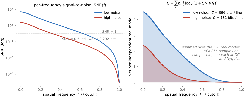
Fellgett and Linfoot Fellgett & Linfoot 1955 and Cox and Sheppard Cox & Sheppard 1986 developed this view for optical imaging. A finite example makes the assumptions and units explicit. Suppose independent real Gaussian scene modes $X_i$ have variances $P_i$, and measurements are $Y_i=s_iX_i+N_i$ with independent Gaussian noise variances $\sigma_i^2$. Then
Each term combines transfer strength, scene power, and noise power. This is mutual information for the specified scene model. Calling it capacity additionally requires maximizing over allowed inputs under a stated power budget. Fourier-domain versions need the correct number of independent modes and spatial normalization; integrating an unspecified SNR curve does not by itself produce a camera’s capacity.
Prior knowledge changes what “resolution” asks of a measurement Toraldo di Francia 1955. Estimating the positions of a known number of point sources differs from recovering an arbitrary scene. Sufficient signal and the correct model can support localization finer than a conventional resolution criterion, without recovering arbitrary frequencies removed by the optics. See Chapter 7.1, Imaging as Bayesian inference with probabilistic priors.
Detective quantum efficiency compares squared signal-to-noise ratios, $\mathrm{DQE}=(\mathrm{SNR}_{\mathrm{out}}/\mathrm{SNR}_{\mathrm{in}})^2$, under a specified signal, photon input, and detector model. Frequency-dependent DQE uses transfer and noise-power measurements. It measures signal-detection efficiency, not Shannon information in bits. The related noise-equivalent quanta, $\mathrm{NEQ}=\mathrm{SNR}_{\mathrm{out}}^2$, is the number of ideal photons that would give the measured signal-to-noise ratio, so DQE is NEQ divided by the photons actually incident. Rose's detectability criterion connects these to seeing: a feature is reliably detected when its signal-to-noise ratio exceeds roughly 5 Rose 1948, which turns a photon count into a prediction of what an observer or a detector can find. The distinction matters when comparing detector performance across tasks; see Part 34, Computational sensors.
7.6.4 Information-theoretic quantities as objectives⧉
Information quantities also provide practical objectives, provided their estimators and assumptions fit the task.
Mutual information can align images from different modalities because corresponding intensities may be statistically dependent without being equal [@viola-wells-1997; @maes-etal-1997]. Alignment is not guaranteed to be the unique maximum: repeated structures, overlap changes, interpolation, and histogram estimation can distort the objective.
Maximum-entropy restoration uses an entropy-related regularizer to select among data-consistent reconstructions [@gull-skilling-1984; @frieden-1972]. One must specify what is normalized into a distribution, and often a positive reference image. Entropy over normalized intensities is different from entropy of a probability distribution over possible images. Positivity, total flux, and the reference model are substantive prior assumptions.
Multiplexing can improve SNR when read noise dominates, but mixing more light also mixes its shot noise; the advantage depends on the noise regime and exposure budget. See Part 33, Computational optics and coded imaging. Plenoptic sampling Chai et al. 2000 (plenoptic sampling) analyzes which rays suffice for alias-free reconstruction under a scene model; see Part 31, Light fields and plenoptic cameras. Neither claim follows from counting measurements alone.
A multimodal pair need not give the same tissue the same brightness. A squared intensity difference then penalizes a correct alignment for a difference caused by the imaging modality. Mutual information instead asks whether the paired values form a statistically informative relationship. In a joint histogram, correctly paired structures may create concentrated relationships even when one modality maps bright tissue to dark. Misregistration mixes unrelated locations and can weaken those relationships. This is the motivation for the criterion, while overlap, repeated patterns, interpolation, and histogram estimation explain why optimization can still fail [@viola-wells-1997; @maes-etal-1997].
7.6.5 The modern revival: learned compression and generative models⧉
Learned codecs optimize the representation and its probability model together.
Ballé and colleagues [@balle-etal-2017; @balle-etal-2018] train an encoder, entropy model, and decoder with an objective $R+\lambda D$. Here $R$ estimates the code length of quantized latent symbols, including side information where used; $D$ measures reconstruction error. Compare actual encoded bytes and quality on held-out images, since an estimated training rate is not necessarily the delivered file size.
For a variational autoencoder, the evidence lower bound is
The first term is a reconstruction log-likelihood, reducing to a scaled squared error only for an appropriate Gaussian observation model. The KL term penalizes deviation of the encoding distribution from its prior Kingma & Welling 2014. Weighting it, as in $\beta$-VAE Higgins et al. 2017 (β-VAE), changes that balance. Code-length interpretations require matching logarithm units and a coding scheme; negative log density for continuous values is not directly a number of bits.
The same structure reads as coding. By the minimum description length principle, the best model of data is the one that describes it in the fewest total bits, model included, and a model's negative log-likelihood is a code length for the data under it; bits-back coding makes the ELBO an achievable code length for a latent-variable model. That reading is why compression and density modeling turned out to be the same problem.
The entropy model is a practical part of the codec. A latent value that the model predicts with high probability can be assigned a shorter code than an unexpected value. A scale hyperprior supplies side information about local latent statistics, improving those predictions at the cost of transmitting the side information itself Ballé et al. 2018 (scale hyperprior). Both costs belong in the rate term. This makes the connection between learning a distribution and saving bytes concrete.
7.6.6 Sampling, sparsity, and histogram entropy⧉
Sampling theorems, sparse recovery bounds, and entropy measures answer related but distinct questions.
The sampling theorem in Chapter 6.4, Sampling, downsampling, and aliasing gives conditions for reconstructing a band-limited signal from samples. It does not specify how many bits a noisy, quantized measurement carries. Compressed sensing exploits restricted signal classes, often sparsity, and has both algorithmic and information-theoretic analyses. A histogram-entropy autofocus score is narrower still: it ignores spatial arrangement and can rise with noise as well as image detail.
7.6.7 Where it is least relevant: aesthetics and perception⧉
Entropy alone does not judge composition, color, or aesthetic value. Information-theoretic optimization can incorporate a perceptual or task-specific criterion, but someone must supply that criterion and establish that it reflects the intended use.
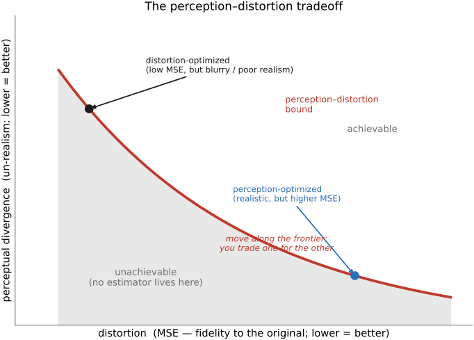
The perception–distortion tradeoff Blau & Michaeli 2018 distinguishes expected error relative to the reference from divergence between the distribution of reconstructions and the distribution of real images. Its achievable bound explains why improving distributional realism can require increased reference error in ambiguous restoration. It is not a theorem that every image has one realism score, or that every algorithm lies on an optimal frontier. When measurements fully determine the source, the ambiguity underlying this tension can disappear.
Use information measures to answer a specified question: code length, dependence on measurements, or a rate–quality tradeoff. State the scene and noise assumptions, the units, and the distortion criterion. More entropy is not automatically a better photograph.