7.3 Deep learning⧉
A learned imaging model can predict restored pixels, a geometric quantity, an edit, or a distribution of possible outputs. These targets require different losses and different evidence of success. Chapter 7.2, Machine learning described the training-data problem; here we examine concrete methods and the choices they illustrate.
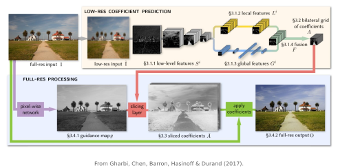
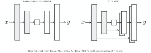
An encoder–decoder gathers context at reduced resolution, then reconstructs spatial output. U-Net skip connections preserve fine input features alongside that context. A model that predicts local color transforms can be much cheaper than one that synthesizes every output pixel; a model that predicts depth instead needs scene-scale cues. Architecture and training details are in Refreshers#Machine learning and deep learning.
7.3.1 Low-level learned operators (pixel-to-pixel)⧉
The standard case is an image-to-image network, typically a U-Net Ronneberger et al. 2015 (U-Net) or encoder–decoder, mapping a degraded or partial image to a restored one. Each task below is a task an earlier chapter solved by hand, now learned from examples instead (Figure 7.3.1).
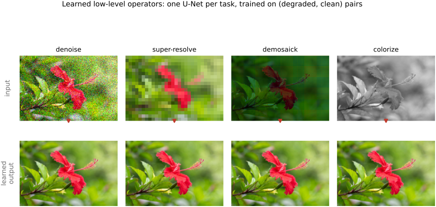
Learned denoisers can outperform classical filters on matching evaluation data, but matching the noise alone does not guarantee performance on unfamiliar content. They can also serve inside plug-and-play reconstruction, subject to compatibility and convergence conditions (Chapter 13.11, Denoising as a universal prior). Diffusion requires a noise-conditioned predictor and a defined sampling schedule (Chapter 7.4, Generative AI and diffusion).
Demosaicking, and joint demosaick-plus-denoise. Gharbi and colleagues (2016) trained a single network to go from a Bayer mosaic straight to full RGB, doing the demosaicking and the denoising at once, on hard cases mined automatically from data. The paper reported improvements over its evaluated classical baselines. This is the headline instance of L7.6: learning the operator end to end beat a long-polished pipeline stage. It is also a quiet argument for jointly learning steps the classical pipeline kept apart, since the net is free to trade off demosaicking against denoising however the data rewards, rather than committing to one before the other the way a fixed sequence must.
Super-resolution. Pose low-resolution → high-resolution as a learned map. This is super-resolution (SR). The lineage runs from Freeman's pre-deep, example-based work (Freeman et al. 2002), which stitched in high-frequency detail copied from a dictionary of patches, through to modern networks: SwinIR (Liang et al. 2021), a transformer restoration backbone, and Real-ESRGAN (Wang et al. 2021), an enhanced super-resolution GAN (ESRGAN) trained against a deliberately realistic model of how real photos degrade so that it survives in the wild. The deep treatment, with priors, lives in Chapter 14.1, What can super-resolution actually do?; here it is one entry in the zoo. When measurements leave ambiguity, the model supplies plausible detail from learned statistics. Note the seam this opens: the actual high-resolution scene is generally not uniquely determined by the input, which is exactly why the strongest super-resolvers reach for the generative machinery later in this chapter.
Colorization, classical and learned, side by side. This task shows the contrast clearly, because two paradigms sit right next to each other (Figure 7.3.2). Levin, Lischinski and Weiss (2004) colorize from a few user scribbles, propagated across the image by optimization under one simple rule: neighboring pixels with similar intensity should get similar color. That rule is an affinity prior, the same edge-aware idea as the bilateral filter (big lesson L10.1), and it is entirely hand-designed; it is also, tellingly, the very matrix-free least-squares solve of Chapter 6.7, Image formation as a linear system, run on color instead of sharpness. Zhang, Isola and Efros (2016) instead learn fully automatic colorization from a huge corpus of color photos stripped to gray and back, posed as classification over quantized colors to keep the output from sliding toward desaturated browns. One propagates a human's chosen colors by a human's chosen rule; the other invents plausible colors learned from millions of images. Same task, opposite philosophies.
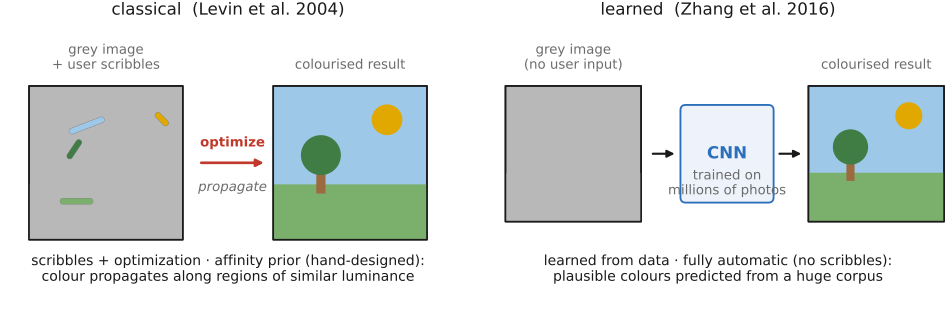
Colorization is also where multimodality matters here. A regression loss tends to produce desaturated, averaged colors because it averages the several colors a gray pixel could plausibly be, so colorization gets its own full treatment, gallery and all, as the single-image part's purest prior-driven recovery (Chapter 24.5, Colorization).
Monocular depth. Estimate depth from a single RGB image. This is badly ill-posed, because one photo is consistent with infinitely many 3-D scenes, so the network must lean hard on a learned scene prior about how the world is usually shaped. MiDaS (Ranftl et al. 2019) trained across many incompatible depth datasets at once with a scale- and shift-invariant loss, so that depth maps recorded in different units could all teach the same net; Depth Anything (Yang et al. 2024) pushed the idea to a massive pile of pseudo-labeled images and got zero-shot depth on photos it had never seen (Figure 7.3.3). Distinguish relative-depth models from models trained or calibrated for metric depth, including metric variants of Depth Anything. Metric prediction uses additional assumptions learned from data; its units do not guarantee correct scale on a new camera or scene. Stereo and dual-pixel depth also require inference, but add geometric measurements.
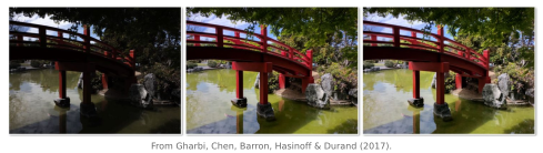
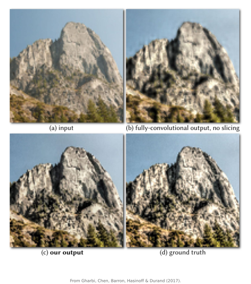
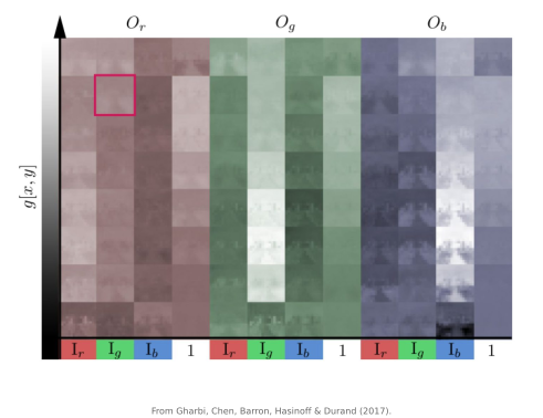
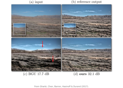
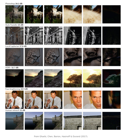
Learned exposure and retouch. Here the "degradation" is taste: learn a photographer's tone and color adjustment from before/after pairs. Bychkovsky and colleagues (2011) built the MIT-Adobe FiveK dataset. It contains the same scenes retouched by five expert editors, which is what made the adjustment learnable at all; the data, once again, is the enabling move. HDRnet (Gharbi et al. 2017) runs fast enough for a phone by predicting not output pixels but the coefficients of a bilateral-grid affine transform, an edge-aware local adjustment (the learned bilateral grid, cross-referenced in the edge-preserving chapter). Exposure (Hu et al. 2018) takes a different and instructive line: it learns a sequence of interpretable operations (curves, white balance, contrast) rather than raw pixels, so the result is an edit a photographer can read and undo. Learn the pixels, or learn the operations: both are on the table, and the choice trades raw quality against the editability and trust of a human-readable result.
7.3.2 Mid- and high-level learned predictors⧉
Not every learned operator outputs an image. A second family predicts semantic structure from a single photo, such as where things are and what they are, and that structure becomes the input to retouching, autofocus, framing, and selection. These are enabling rather than central, so we keep them brief.
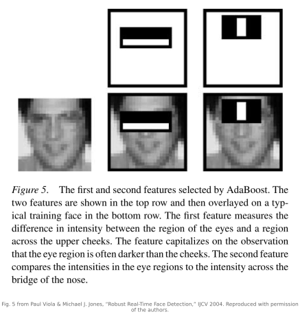
Sky and face detection are the classic "where is the sky, where are the faces" predictors that drive auto-enhance and metering: brighten the faces, deepen the sky, expose for the subject. The lineage runs from pre-deep detectors of the Viola–Jones era (Viola & Jones 2004, the cascade of simple features that first made real-time face detection practical) to modern networks; the point for us is that semantic masks let a retouching pipeline apply different adjustments to selected subjects.
Face landmarks and pose estimate keypoint positions and head orientation for portrait editing and augmented reality. Geometric inconsistencies can be one forensic cue, but plausible landmarks do not authenticate a photograph (Chapter 40.2, Ethics of computational photography).
Saliency and gaze prediction estimate where people look in an image. Pre-deep models built saliency from hand-designed contrast features. The classic Itti, Koch and Niebur (1998) model combined center-surround contrasts of color, intensity, and orientation into one saliency map, while learned models train directly on eye-tracking data. The uses are practical: auto-cropping and reframing, retargeting, aesthetics scoring, and attention-aware compression that spends bits where the eye will actually land.
7.3.3 Generative models: image-to-image translation⧉
Sometimes there is no single correct answer. Ask a network to colorize a gray photo, super-resolve a tiny one, or fill a hole, and many different outputs are equally plausible. The task is one-to-many. Regression handles this badly: minimizing squared error pulls the network toward the average of all plausible answers, and the average of many sharp images is a blurry one. (We pin down exactly why that average looks bad yet scores well when we reach metrics, below.) The cure is to stop averaging and start sampling: model the space of plausible answers and draw one sharp, plausible member. That is the shift from regression to generative modeling.
GANs. A generative adversarial network (GAN) pits two networks against each other: a generator proposes images while a discriminator learns to tell real from generated. Train them in opposition and the generator is pushed to produce output the discriminator cannot distinguish from real, which encourages sharp, plausible detail rather than a blurry mean. This adversarial training (Goodfellow et al. 2014) is the engine behind Real-ESRGAN's realism. We give it one paragraph of intuition; the full generative story, and why diffusion has largely displaced GANs, is Chapter 7.4, Generative AI and diffusion.
The catch with clever losses. The reason to reach for an adversarial or perceptual loss is exactly the one from big lesson L13.4: a plain $L_2$ loss returns the average of plausible answers, so to get sharp, believable detail you must score plausibility instead, with a learned discriminator (GAN) or a deep-feature distance (a VGG/perceptual loss, or LPIPS). But every step away from a simple, fixed loss toward a complex, learned one buys that realism at a real cost, and the main failure modes are: Training gets unstable: the GAN's two networks chase a moving target, and the equilibrium is delicate. If the discriminator is too strong, the generator's gradients vanish. If it is too weak, the generator learns little. It hallucinates: a loss that rewards "looks real" will happily invent texture, teeth, or text that was never in the input, producing detail that is plausible, sharp, and wrong, which is fine for a pretty photo and dangerous for evidence or medicine. It can collapse to a few safe outputs (mode collapse). And a learned loss is a network, and networks can be gamed: the generator learns to exploit the discriminator's blind spots rather than to improve. This is Goodhart's law again (big lesson L9.4). The moment your measure of quality becomes the target you optimize, it stops measuring quality. The practical disciplines all follow from this: combine the adversarial term with a stabilizing reconstruction term rather than using it alone, keep a held-out evaluation (or a human study) you never trained against, and treat any sharp detail a complex loss produces as a hypothesis about the scene, not a measurement of it.
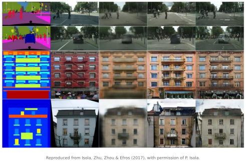
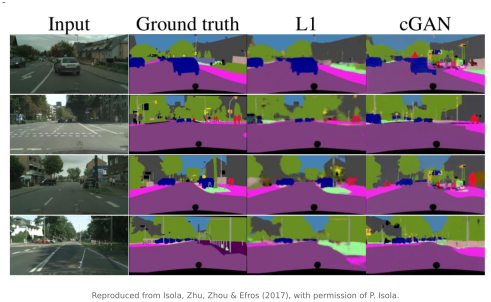
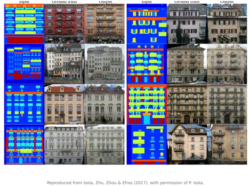
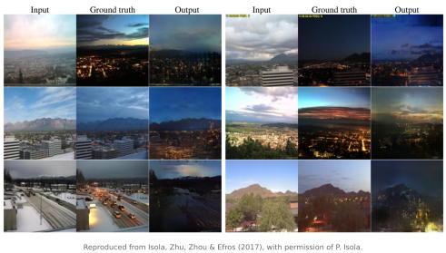
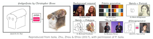
Conditional translation, paired and unpaired. Pix2Pix (Isola et al. 2017) is the generic tool: a conditional GAN that learns to map one image domain to another from paired examples: edges→photo, label-map→street scene, day→night (Figure 7.3.15). When you have no aligned pairs, CycleGAN (Zhu et al. 2017) does the unpaired version, encouraging round-trip reconstruction with a cycle-consistency constraint (translate there and back and you should land where you started): horses↔zebras, summer↔winter, photo↔painting, all without a single matched pair.
The CycleGAN paper's own results show what unpaired translation, held together by cycle consistency, can do.
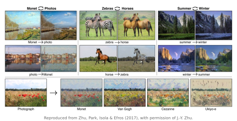
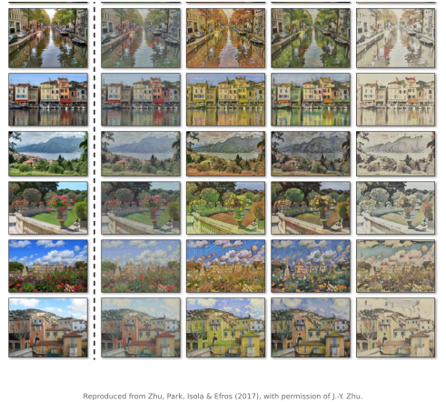
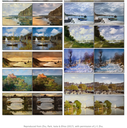
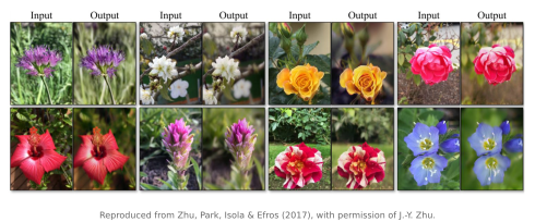
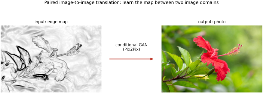
The Pix2Pix and CycleGAN papers' own figures make the generality, the mechanism, and the role of the adversarial loss concrete.
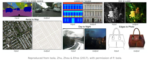
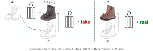

The pre-deep ancestor. "Translate one image into the style of another" predates deep nets. Image Analogies (Hertzmann et al. 2001) learned a filter from a single example pair (given A and its filtered version A′, apply the same transformation to a new B to get B′) by matching patches. The same instinct as Pix2Pix ("A is to A′ as B is to B′"), using a nonparametric patch model instead of a trained deep network (ties to the texture-synthesis and patch-matching material).
Chapter 7.4, Generative AI and diffusion develops noise-based generative models and their use for conditioning on text, images, or physical measurements.
7.3.4 Learned perceptual metrics and losses⧉
There is a question we have been deferring: how do we measure whether a restored or generated image is any good? The answer matters more than it sounds, because the metric you optimize quietly defines what "good" means. The classical metrics break exactly where learned methods are supposed to shine.
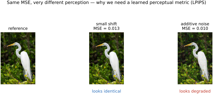
MSE and PSNR compare aligned pixel values. They are useful for reconstruction fidelity, but do not fully predict perceived similarity: a small displacement of a texture can produce a large pixel error. SSIM compares local structure, and visual-difference predictors explicitly model aspects of perception, so they should not be grouped as metrics “blind to texture.” The appropriate metric depends on whether exact position, perceived quality, or semantic similarity matters (Chapter 9.3, Image metrics).
A feature loss compares intermediate activations of a fixed network:
LPIPS Zhang et al. 2018 normalizes the feature vector across channels at each spatial location, then weights squared channel differences and averages spatially. Writing these normalized vectors as $\bar\phi_l$,
The weights $a_{l,c}$ are fitted to human judgments. This is distinct from a plain feature loss. Features remain spatially indexed; LPIPS is not invariant to arbitrary shifts. State the backbone, preprocessing, and version when reporting scores.
DreamSim Fu et al. 2023 compares whole-image embeddings and is trained on human judgments of synthetic image triplets. It captures differences in layout, pose, color, and semantic content that local patch metrics can miss. It measures a different range of similarities; it is not a universal replacement for LPIPS or a test of photographic truth.
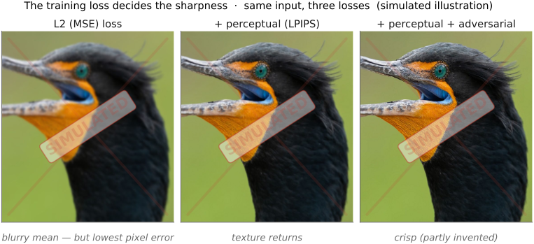
From metric to loss: how perceptual losses buy sharpness. This matters in practice because the metric you train against decides what the network produces. Train a restoration or super-resolution network to minimize per-pixel MSE and it learns to hedge: when several sharp outputs are all plausible, the single image that minimizes average pixel error is their blurry mean, so MSE-trained networks systematically wash out fine texture (Figure 7.3.26). Swap in, or add, a perceptual (feature) loss: push prediction and target through a fixed pretrained network and penalize the distance between their deep features (the plain feature loss, or LPIPS), rewarding the network for reproducing texture and structure rather than exact pixels, so it stops fearing detail it cannot place pixel-perfectly. Add an adversarial (GAN) term, a discriminator trained to tell restored from real, and the output is pushed onto the manifold of real images, crisper still. The caveat is the perception–distortion tradeoff: the sharper and more "real" you push, the more the model invents detail that may not be true; the extra sharpness is bought partly with hallucination, which is why a fidelity anchor stays in the mix.
A combined objective can include pixel, feature, and adversarial terms:
There are no portable default weights: their scale depends on image normalization, sum versus mean reduction, feature layers, and the adversarial formulation. L1 targets a conditional median, whereas L2 targets a conditional mean. Either can lose uncertain texture. A pixel term encourages agreement with the training target; it is not a hard measurement constraint.
Choose the loss for the use case. Compare pixel fidelity, perceptual scores, data residuals when applicable, and representative held-out images. A metric used for training is insufficient as the sole evaluation. Inspect text, repeated patterns, faces, fine structures, and out-of-distribution content for invented detail.
A small translation illustrates the difference between pixel and feature comparisons. Two photographs can show nearly the same content while an edge moves by a pixel, producing a large set of pixel differences. A feature representation can be less sensitive to that displacement, which can make it useful for judging appearance. That tolerance is also a limitation when exact alignment matters. Combining a pixel loss with a feature loss makes the tradeoff explicit; the weights determine how strongly the training penalizes each kind of disagreement.
The terms in a combined loss serve different purposes. A pixel term penalizes color and spatial disagreement with the reference. A feature term penalizes disagreement in the chosen representation of texture and structure. An adversarial term favors outputs that the discriminator treats as belonging to the reference distribution. Inspect their numerical magnitudes and gradients under the actual normalization before choosing weights. Increasing the adversarial contribution can improve appearance while weakening correspondence to the particular captured scene; no coefficient range alone defines a safe balance.
Learning has now entered both sides of the experiment: the operator that makes an image and the metric used to judge it. The second learned model brings its own training examples and invariances. Agreement between the two models can therefore reflect shared assumptions rather than independent evidence of success. This is why the evaluation should retain measurements or human judgments that were not used to fit either model.