6.6 Pyramids and wavelets⧉
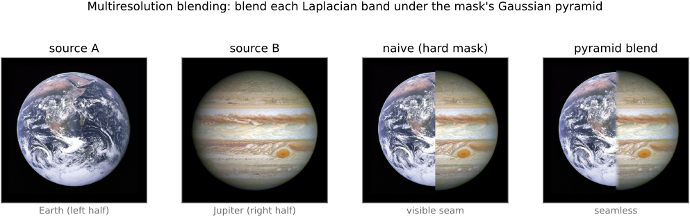
Picture this problem. You have a photograph of Earth and a photograph of Jupiter, and you want to join the left half of one to the right half of the other so smoothly that nobody can find the seam. Try the obvious thing, cut both down the middle and paste, and a hard line runs down the join: every detail, coarse and fine, changes at one pixel. Try to hide that line by blurring across the boundary, and now you have smeared Earth's coastlines into Jupiter's cloud bands; the broad colors finally cross-fade, but the fine texture has turned to mush. Neither works because each uses a single scale of blending. What the picture actually needs is to blend gently where it is smooth (the slow sweep of color across the two disks) and sharply where it has detail (the cloud bands, the coastlines) at the same time. A single blur cannot do that, because a blur has one width. The moment we stop treating the image as one thing and start treating it as a stack of things at different scales, the problem becomes manageable.
That stack is what this chapter is about. We will build a multiresolution representation of an image, a tower of versions running coarse to fine, and then learn to split it into overlapping bands of detail that we can edit one at a time. The result is a representation that is local in both space and frequency, the very combination the Fourier chapter told us we could not get for free. Most of the chapter is spent on the two classic constructions, the Gaussian pyramid and the Laplacian pyramid of Burt and Adelson; we close with their principled relatives, wavelets and steerable pyramids.
6.6.1 Halfway between space and frequency⧉
Name the problem up front, because it is the same one the whole back half of basic image processing keeps circling. So far we have two ways to represent an image, and each is perfect at one thing and useless at the other. In the primal domain a pixel is a value at a place: perfectly local in space, but with no notion of scale: it cannot tell you whether you are looking at a broad gradient or a fine edge. In the Fourier domain a coefficient is the amount of one sine wave: perfectly local in frequency, telling you exactly which scales are present, but each coefficient is spread over the entire image, with no notion of where.
The complete Fourier transform retains spatial information, but a single coefficient describes a wave spanning the whole image. Pyramids put each scale’s responses on a spatial grid, which makes local editing easier. Their boundary rules still need to be specified, just as they do for convolution.
The Fourier chapter's lesson was diagonalize when you can: work in the basis where your operator is simple. This chapter adds the practical sequel: the perfect basis is rarely the useful one. Fourier is perfectly localized in frequency and not at all in space; the primal grid is the reverse. The uncertainty principle (compact in space ⇔ spread in frequency, from the Fourier chapter) says you cannot have both perfectly. A pyramid surrenders a little of each (it chops frequency into a few coarse bands and keeps each band laid out spatially), and that modest sacrifice is exactly what makes per-scale, per-region editing possible. Reach for a representation that is local in both, not for the one that is perfect in one.
6.6.2 The idea: process an image at many resolutions⧉
The core idea, due to Peter Burt and Edward Adelson in the early 1980s, is simple: represent the image at several resolutions at once, and handle each scale on its own. A coarse version holds the broad layout: the overall light, the large shapes. A fine version holds the texture and the edges. Once you can reach into each scale independently, a startling range of operations falls out nearly for free: blending (Earth and Jupiter), denoising, tone mapping, compression, feature analysis, coarse-to-fine motion estimation, and, much later in the book, the pooling layers and U-Nets of deep networks. We will preview several of these at the end and develop them properly in their own chapters; the point for now is that they are all the same trick wearing different hats.
There are two flavors of pyramid, and the difference maps cleanly onto frequency. A low-pass pyramid stores, at each level, a lower-resolution copy of the whole image: that is the Gaussian pyramid. A band-pass pyramid stores, at each level, only a narrow band of frequencies (the detail one scale adds over the next coarser one), and that is the Laplacian pyramid. We build the low-pass one first, because the band-pass one is simply the differences between its levels.
6.6.3 The Gaussian pyramid⧉
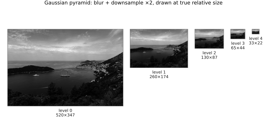
Begin with the original image. Blur it with a small Gaussian, then throw away every other pixel in each direction, so the result is half as wide and half as tall, a quarter of the pixels. Do the same to that image, and again, and again, until you are down to a handful of pixels. The sequence of ever-smaller, ever-coarser images is the Gaussian pyramid, and stacking them smallest-on-top is what earns it the name (Figure 6.6.1). We write the levels $G_0$ (the original, full resolution), $G_1$, $G_2$, and so on, each $G_{k+1}$ one octave coarser than $G_k$.
The blur-then-downsample step has a name, the reduce operator: $G_{k+1} = \text{reduce}(G_k)$, where reduce means "blur with a small Gaussian, then drop every other sample." The blur is not optional. We are halving the sampling rate, and Chapter 6.4, Sampling, downsampling, and aliasing, was emphatic that you must low-pass before you downsample, or you alias: moiré and jaggies folded in from the frequencies the coarse grid cannot represent. The Gaussian is the prefilter; downsampling by two is the resample. So a pyramid level is not "the image, smaller," it is "the image with its highest frequencies attenuated, then sampled at the rate that octave-removed image deserves."
Expansion predicts a fine level from the next coarser one. One concrete implementation uses the separable binomial filter $h=[1,4,6,4,1]/16$. Reduce by filtering with $h$ in both axes and retaining samples at even indices. Expand by inserting zeros at the missing positions and filtering with $2h$ along each axis, or $4(h\otimes h)$ in 2-D. The gain compensates for the inserted zeros and preserves a constant image in the interior. Use the same boundary extension and pixel alignment throughout.
Expand is a prediction, not an inverse of reduce. It need not pass through the coarse samples. For odd image dimensions, pass the target fine-level shape explicitly and crop to that shape.
You might worry that storing the image at every scale balloons the memory. It barely does. Each level has a quarter of the pixels of the one below ($1 + \tfrac14 + \tfrac1{16} + \tfrac1{64} + \cdots$), and that geometric series sums to 4/3. The entire Gaussian pyramid, from full resolution down to a single pixel, costs only about a third more storage than the original image. Coarse-to-fine search, scale-space analysis, and everything else in this chapter ride on that bargain.
6.6.4 The Laplacian pyramid⧉
The Gaussian pyramid is useful but redundant in an unsatisfying way: each level repeats most of the information already in the level below, just blurrier. The interesting question is not "what does the image look like coarse" but "what does each scale add." That is what the Laplacian pyramid captures, and it is built straight out of the Gaussian one.
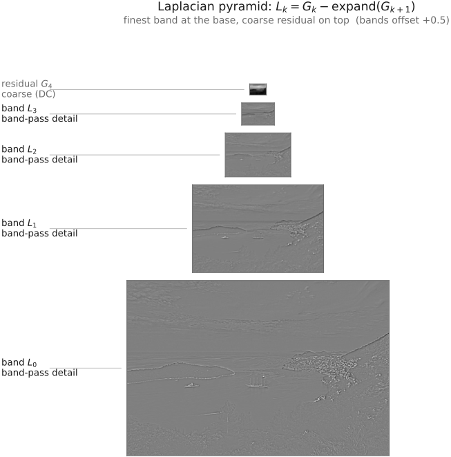
Take a Gaussian level $G_k$. The next coarser level $G_{k+1}$ is a blurred, shrunk version of it; expand it back up to $G_k$'s size and you get a smooth prediction of $G_k$, everything except the finest octave of detail, which the blur removed. Whatever $G_k$ has that this prediction lacks is exactly the band of detail that this scale contributes. So subtract:
That difference image, $L_k$, is the Laplacian pyramid level $k$ (Figure 6.6.2). It is band-pass: it holds neither the broad low frequencies (those survived into $G_{k+1}$ and got subtracted away) nor any frequencies too fine for $G_k$ to represent: mainly the detail between those scales, with overlapping responses rather than sharp octave boundaries. Read the equation back in words: each Laplacian level is what one Gaussian level has that the next coarser one, blown back up, is missing. The coarsest level of the whole structure is special (there is no coarser Gaussian to subtract), so we keep the smallest Gaussian image $G_n$ itself as the apex, a tiny low-pass residual carrying the average brightness and the very largest-scale variation.
The name is a small piece of history. Expanding $G_{k+1}$ and subtracting it from $G_k$ is, up to scaling, a difference of Gaussians (one blur minus a slightly bigger blur), and a difference of Gaussians is a well-known approximation to the Laplacian operator, the thing that measures how much a pixel differs from the average of its neighbors. So each Laplacian coefficient behaves like a local second derivative: near zero in flat regions, large at edges and texture. Hence "Laplacian pyramid."
6.6.5 Reconstruction: an exact encoder and decoder⧉
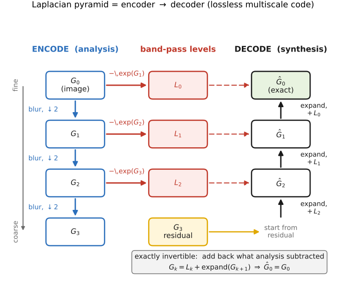
Here is the property that turns the Laplacian pyramid from a curiosity into a workhorse: it loses nothing. We can put the image back together exactly. Just rearrange the construction equation. We defined $L_k = G_k - \text{expand}(G_{k+1})$, so
Read this as a recipe that climbs from coarse to fine. Start at the apex with the residual $G_n$. Expand it and add the band-pass level $L_{n-1}$ to recover $G_{n-1}$. Expand that and add $L_{n-2}$ to recover $G_{n-2}$. Keep going one level at a time, and the last addition hands you back $G_0$, the original image, pixel for pixel. The build (analysis) and collapse (synthesis) are the two loops, one the exact inverse of the other:
# analysis: build the Laplacian pyramid
G[0] = im
for k in 0 .. n-1:
    G[k+1] = reduce(G[k])               # blur, then downsample by 2
    L[k]   = G[k] - expand(G[k+1], shape(G[k]))  # band-pass detail at scale k
# L[0..n-1] plus the residual G[n] are the pyramid

# synthesis: collapse it back, coarse to fine
out = G[n]                              # the low-pass residual
for k in n-1 .. 0:
    out = L[k] + expand(out, shape(L[k])) # undo each subtraction
return out                              # equals the original, up to round-off
The reconstruction is exact up to round-off because each stored residual undoes the same prediction used in analysis. The prediction itself can be approximate. Quantizing or clipping residuals, changing the expansion filter, or changing its boundary rule breaks this identity. Store signed floating-point coefficients while editing.
This is the encoder–decoder framing, and it is the right way to hold the whole construction in your head. Building the Laplacian pyramid is the encoder (or analysis): it takes the image apart into scale bands. Reconstructing is the decoder (or synthesis): it puts them back. The two are exact inverses, which is precisely what licenses the central move of this chapter: edit the bands in the middle. Because each $L_k$ isolates a range of detail scales, you can darken one, amplify another, zero a third, then run the decoder, and you get a coherent image back with no seams between scales. Blending, coring, detail enhancement, and tone mapping are all just different things to do to the bands before re-synthesizing.
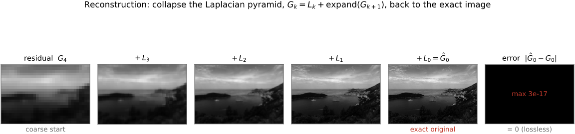
Seeing it run on real pixels makes the "loses nothing" claim concrete. Start from the coarse residual, a tiny, blurry image with only the broadest tone, and add the bands back one octave at a time: the picture sharpens from broad light, to coarse structure, to fine edges and texture, until the last band hands back the original. Subtract that reconstruction from the original and the difference is flat black, exactly zero, up to floating-point round-off (Figure 6.6.4).
6.6.6 Each level is a frequency band⧉
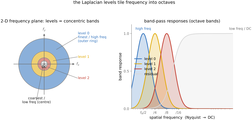
Each Laplacian level responds most strongly to a range of spatial frequencies, roughly an octave apart from the adjacent level. Draw these as overlapping bands, not disjoint rings. Downsampling also makes the response depend on sampling phase. Exact reconstruction follows from the residual equation, not from a perfect partition of the Fourier plane.
But, and this is the entire point, within each band the information is still laid out spatially. The Laplacian level is an image: it tells you not only which frequencies are present but roughly where in the picture they live. That is the local-in-both property we have been chasing. The cost is that the frequency bands are crude (a handful of octave-wide rings rather than Fourier's per-frequency precision), and the price of spatial locality is some smearing of frequency, exactly as the uncertainty principle demands. A Laplacian pyramid is a deliberately coarse carving of frequency into bands, with the position within each band left spatial: a sensible middle of the road between the primal grid and Fourier.
6.6.7 What the bands look like on a real image⧉
On natural photographs, Laplacian coefficients usually have a strong concentration near zero and a long tail of larger responses at edges and texture. Near zero does not mean exactly zero, and edges commonly produce responses at several scales. The transform reduces some pixel correlations but does not make coefficients independent. Smooth local ramps give small responses away from boundaries when the filters reproduce constants and linear trends.
Thresholding exploits this concentration, but small coefficients include weak real texture and large coefficients can include noise. For white pixel noise of variance $\sigma^2$, a coefficient formed with effective weights $h_i$ has noise variance $\sigma^2\sum_i h_i^2$. Different levels therefore need different noise scales, and their noise is generally correlated. Chapter 2.8, Noise, signal-to-noise ratio and dynamic range describes the sensor model; the denoising chapters develop coefficient shrinkage.
Inspect a smooth sky and a textured roof in one Laplacian level. Many sky coefficients lie close to zero, while roof edges produce larger positive and negative values. Quantization can spend few bits on the small values; a denoiser can reduce them when they are more likely to be noise. But a weak real texture also produces small coefficients, and noise can produce large ones. The sparse histogram motivates both operations without identifying signal and noise perfectly. Looking across neighboring locations and scales provides evidence that the coefficient magnitude alone lacks.
6.6.8 Limitations⧉
A Laplacian pyramid stores approximately $4/3$ as many coefficients as pixels. It is redundant; redundancy and the mathematical property of being a tight frame are separate questions. Downsampling makes coefficients sensitive to a one-pixel translation, especially at coarse levels. Standard Laplacian levels have no separate orientation channels, but their spatial patterns still distinguish horizontal and vertical edges. Separable filters are only approximately isotropic.
6.6.9 Cousins: wavelets and steerable pyramids⧉
The Laplacian pyramid was the first of a family, and its siblings each fix one of those limitations.
A critically sampled wavelet transform can keep one coefficient per input sample. The simplest example, Haar, replaces a pair $(a,b)$ by its normalized average and difference:
Applying this along rows and columns produces a low-pass band and three detail bands; recursively transform the low-pass band. Orthogonal wavelets preserve energy. Biorthogonal wavelets use different analysis and synthesis filters and can also reconstruct exactly; JPEG 2000 uses this family. Undecimated wavelets deliberately retain redundancy to improve translation behavior. “Wavelet” therefore does not by itself mean a nonredundant orthogonal basis.
It helps to see the three representations on one axis. Pure Fourier is all frequency, no space: each basis function is a sine wave filling the image. The pure primal grid is all space, no frequency: each basis function is a single pixel. Wavelets and pyramids sit in between: each basis function is a little bump, somewhat localized in space and covering a band of frequencies, and you can even dial where they sit, trading spatial sharpness for frequency sharpness. This is the same uncertainty tradeoff from the Fourier chapter, now offered as a design knob rather than a fixed pair of extremes.
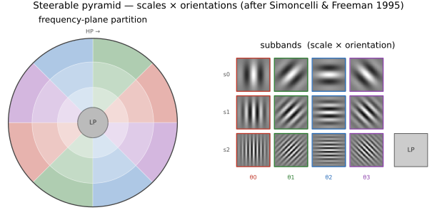
Steerable pyramids (Simoncelli and Freeman, 1995) go the other way and add back what the Laplacian pyramid lacks: a notion of orientation. They split each frequency band further into a few oriented sub-bands (horizontal, vertical, diagonal) so the representation captures not just the scale of a feature but its direction, and does so in a way that is translation- and rotation-equivariant in the ideal construction: responses move with a translated image and can be steered to new orientations. The price is even more overcompleteness. They are the tool of choice when orientation matters: texture analysis, and the phase-based video magnification we will meet later. (There is also multigrid, a coarse-to-fine relative from numerical analysis used to solve large linear systems fast, which we mention only in passing.)
Choose a Laplacian pyramid for simple multiscale editing, critically sampled wavelets when coefficient count matters, and an oriented representation when the application needs scale and direction. The redundancy, filters, and sampling scheme determine their behavior under translation.
6.6.10 Pyramid blending⧉
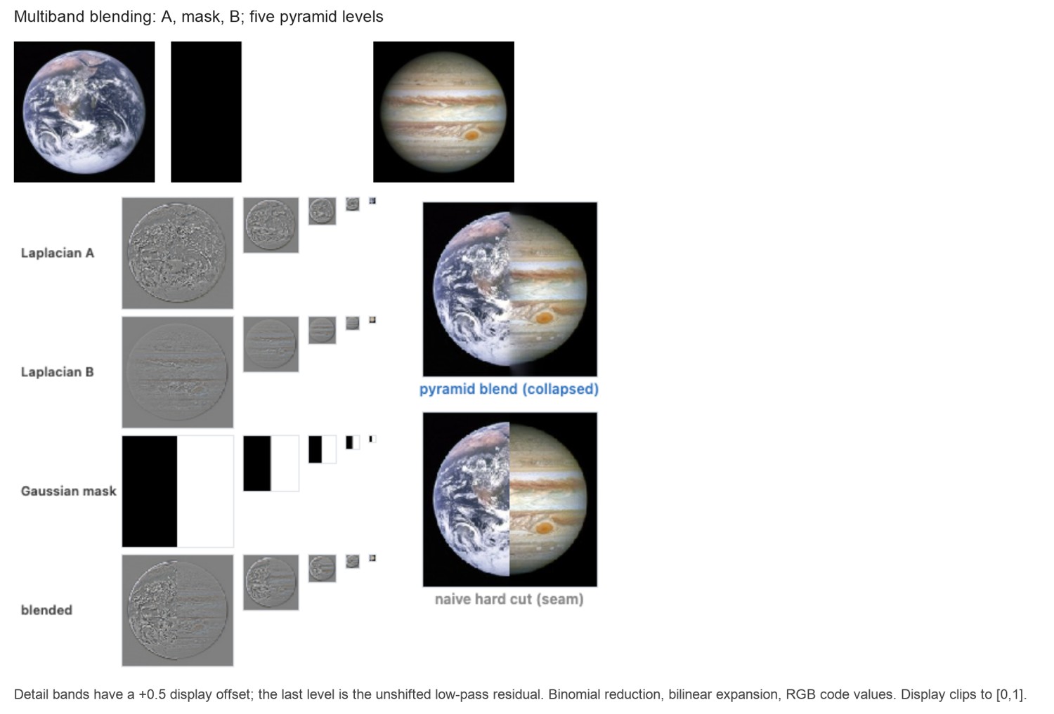
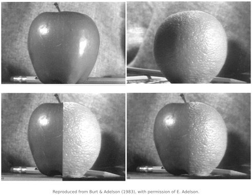
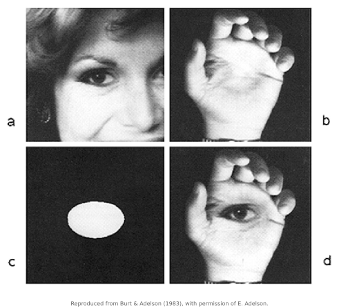
We have built the representation; the rest of the book spends it, and the original application, still the iconic one, is multiscale blending, the Earth and Jupiter we opened with (our pedagogical stand-in for Burt and Adelson's own motivating result, the apple-and-orange "orapple" of Figure 6.6.9). The recipe: build a Laplacian pyramid of each source image and a Gaussian pyramid of the mask that says where to switch from one to the other; then, level by level, mix the two source bands using the mask at that scale,
blend the coarsest Gaussian residuals with the coarsest mask as well, and finally run the decoder on the blended pyramid (Figure 6.6.7). The key detail is that the mask gets its own Gaussian pyramid, not a Laplacian one: $\text{mask}_k$ is the mask blurred and shrunk to level $k$, so it is broad and soft at the coarse levels and crisp at the fine ones. The transition is therefore wide for the low frequencies and narrow for the high ones: a gentle cross-fade of the broad colors, a crisp switch of the fine texture. That is exactly the "blend smoothly where smooth, sharply where detailed" we wanted and could not get from a single blur. The full treatment is in compositing and panorama chapters.
Better still, drive the whole construction and watch every pyramid (Figure 6.6.8).
Because this blend runs over the values band by band, it keeps each source's own brightness (its DC) and merely feathers the two across the mask. That is exactly what sets it apart from the gradient-domain Poisson blend, which discards the source's level and re-derives it from the boundary; the two are placed side by side, including the revealing case of pasting a constant, in Chapter 10.8, Poisson image editing.
6.6.11 Other applications optional⧉
Blending is the headline use, but the same decomposition powers several more, each developed properly in its own chapter, and each a different way of spending the band-by-band, scale-local view a pyramid gives.
Exposure fusion merges several differently-exposed shots of one scene the same way, taking each pixel from whichever exposure renders it best and stitching the choices together across scales so there are no seams. Chapter 18.4, Exposure fusion develops it, weights and all.
Coring denoises an image by shrinking the small detail coefficients of each band, where noise dominates, while keeping the large ones that edges and texture produce, then collapsing the pyramid. Chapter 13.4, Pyramid and wavelet denoising develops it: the shrinkage curves, how to set a threshold per band, and the statistical models that refine them.
Local Laplacian filtering (Paris, Aubry and colleagues, 2011–2015) is the modern, edge-aware extreme: it manipulates the Laplacian coefficients with a per-pixel nonlinearity to boost detail or compress range without the halos a naive high-frequency boost produces. Its edge-aware remapping differs from applying one fixed scalar shrinkage curve to every band coefficient. We develop it (and show the authors' video) in Chapter 10.4, Local Laplacian filters; here it stands as proof that this 1980s representation is still doing frontline work.
6.6.12 Coarse-to-fine methods⧉
Coarse-to-fine motion estimation reduces large displacements before refinement, though a coarse level can lose small objects. Scale-space detectors search across blur levels; a basic octave pyramid needs additional within-octave scales for fine scale selection. U-Nets also combine coarse context with fine spatial features, but their learned encoder and decoder are not guaranteed inverses. Increasing channel counts also changes the $4/3$ storage calculation.
Recap: big lessons of this chapter
The Fourier chapter's lesson was diagonalize when you can: work in the basis where your operator is simple. This chapter adds the practical sequel: the perfect basis is rarely the useful one. Fourier is perfectly localized in frequency and not at all in space; the primal grid is the reverse. The uncertainty principle (compact in space ⇔ spread in frequency, from the Fourier chapter) says you cannot have both perfectly. A pyramid surrenders a little of each (it chops frequency into a few coarse bands and keeps each band laid out spatially), and that modest sacrifice is exactly what makes per-scale, per-region editing possible. Reach for a representation that is local in both, not for the one that is perfect in one.