6.5 Resampling and upsampling⧉
Resizing an image is routine: shrink a photo for the web, zoom into a crop, straighten a tilted horizon, or undo lens distortion. It feels like it should be a one-liner. To make a picture twice as big you spread the pixels out; to make it smaller you throw some away. The whole point of this chapter is that both of those instincts are wrong, and that doing the job well, well enough that repeated rotations do not degrade the image badly, depends on everything we built in Chapter 6.2, Convolution and Chapter 6.3, Fourier, and on the sampling theory of Chapter 6.4, Sampling, downsampling, and aliasing.
The recorded pixels sample an image already filtered by optics and pixel integration. Resizing asks for values on a new grid. We first reconstruct a continuous approximation from the available samples, then filter it for the new grid and sample it there. Interpolation chooses that approximation; it cannot identify arbitrary unrecorded detail.
6.5.1 Domain operations: moving pixels around⧉
Recall the three families of image operation from Chapter 8.3, Tone point operations, sorted by what each output pixel is allowed to read. Resampling is the domain family: the underlying continuous image is remapped in position; discrete resampling generally blends its recorded colors. Formally a domain transform applies a function $f$ from the plane to itself (from $\mathbb{R}^2$ to $\mathbb{R}^2$) to the image's coordinates, with the rule that if the point $(x,y)$ carried color $c$ in the input, then $f(x,y)$ carries that same color $c$ in the output. The range (the colors) is untouched; only the domain (the coordinates) is remapped.
That one definition spans a huge amount of ground. When $f$ is a uniform scale it is resizing; a rotation straightens a horizon; an affine or perspective $f$ fixes keystoning or stitches a panorama; and a freely chosen $f$ is a warp: picture the image printed on rubber and stretched. The free-form case, including how a user even specifies such an $f$ (and the morphing it unlocks), gets its own Chapter 11.2, Antialiasing for complex transforms. Here we take $f$ as given and concentrate on the hard part shared by every domain transform: the new positions almost never land on the input grid, so we must invent values between the samples.
6.5.2 Start with scaling up⧉
Start with the friendliest case, scaling an image up, say by an integer factor $k$. The output has $k$ times as many pixels along each axis, so most output pixels sit between input pixels and have no value of their own: we have too few samples and must fill in the gaps. (Downsampling is the opposite complaint, too many input samples crowding into each output pixel, and, surprisingly, it needs a slightly different fix. Hold that thought; the machinery is almost identical.) Upsampling is the cleaner place to build intuition, so we begin there.
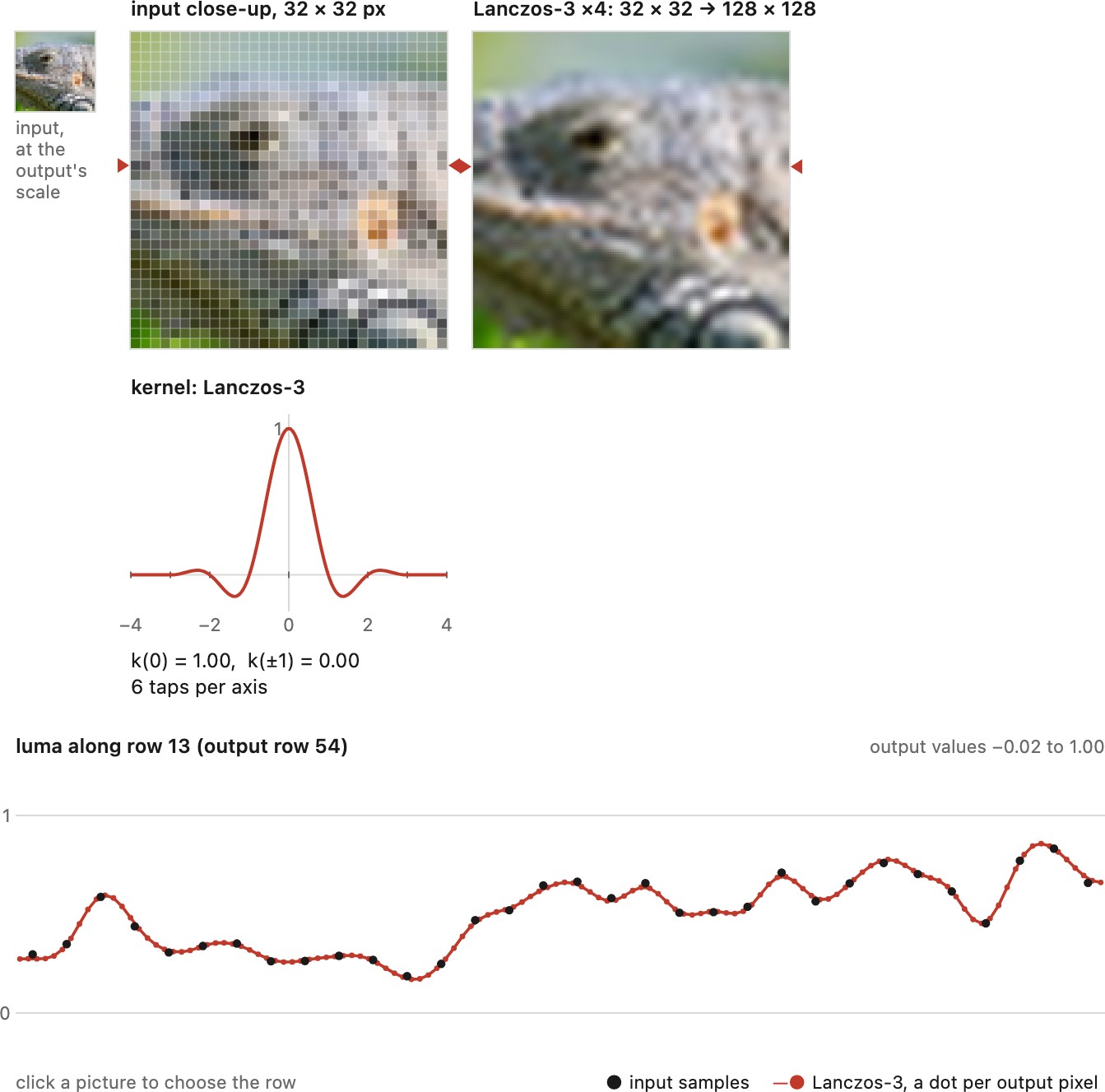
Figure 6.5.1 follows one small image through every method of this chapter, one stage per method; its first stage is the input itself.
6.5.3 The naive idea, and why it leaves gaps⧉
Here is the instinct nearly everyone has first: loop over the input pixels, and for each one compute where it lands in the output and write its color there. To scale up by $k$, the input pixel at $(x,y)$ goes to output location $(k\,x,\ k\,y)$:
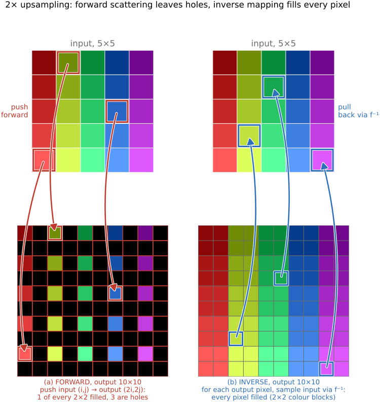
This is forward mapping: push each input pixel forward to its destination. It is intuitive, and it is broken. Scale up by $k=2$ and you write output pixels $(0,0),(2,0),(4,0),\dots$ while every odd-coordinate pixel is never touched: a regular lattice of black holes (Figure 6.5.2, left). The output is mostly gaps, because spreading $N$ input pixels over $k^2 N$ output positions can fill at most $N$ of them: one cell of every $2\times2$ block, three left empty.
You might try to patch it with an inner loop that paints the little square between four placed pixels. That limps along for an axis-aligned enlargement, but the instant $f$ is a rotation the gaps stop being neat squares: they become slivers at odd angles, and "fill the gap" no longer has an easy shape. Forward mapping fights you. We need a different loop.
The second stage of Figure 6.5.1 runs this naive loop on a real image.
6.5.4 Loop over the output, use the inverse transform⧉
The fix is to turn the loop inside out. Instead of pushing inputs forward, iterate over the output pixels (all of them, so none can be skipped) and for each one ask where did this come from in the input? That means applying the inverse transform $f^{-1}$ to the output coordinate and reading the input there:
For a scale-up by $k$ the inverse divides by $k$, so output pixel $(x,y)$ reads the input at $(x/k,\ y/k)$. Now every output pixel receives exactly one value and there are no gaps by construction. This is inverse mapping: loop over output pixels and use the inverse transform when it exists. An occlusion, a fold, or a location outside the source also needs an explicit visibility or boundary rule. It is the same "where-from, not where-to" reflex as the flip in convolution (to fill a destination, reach back into the source), and it is the single most important habit in this chapter. (Figure 6.5.2 sets the two loops side by side.)
Loop over output pixels and pull back through $f^{-1}$ to find where each one reads from. Gathering fills every output exactly once; scattering pushes input pixels forward and leaves holes whose shape depends on the transform, a lattice of gaps under a scale and tilted slivers under a rotation. The same reflex governs warping, morphing, texture mapping, and flow-based reprojection later. Scattering earns its place only when the forward map is the thing you actually have, as in splatting a point cloud, and then it needs an explicit accumulation and normalization pass.
There is one immediate wrinkle, and it is the real subject of everything that follows. Inverse mapping is clean, but $f^{-1}(x,y)$ lands at a fractional coordinate: $(x/k,y/k)$ is rarely an integer, and under a rotation it essentially never is. There is no pixel sitting at $(1.3, 4.7)$. So the genuine content of resampling is the question we have been circling: given the input samples, what value should we report at a position between them? Every method below is one answer.
6.5.5 Nearest neighbor⧉
Round the fractional coordinate to the nearest sample and copy its value. At $1.3$, return $I[1]$; at $1.8$, return $I[2]$. Truncating the coordinate instead gives a different, biased convention. Nearest neighbor is appropriate for categorical labels and for deliberately showing the original pixels, but looks blocky on photographs.
It works and it is fast, but the result is conspicuously blocky: a whole range of fractional positions all snap to the same input pixel, so an upscaled image looks like fat rectangular tiles (Figure 6.4.16, nearest panel), each input pixel becoming a hard $k\times k$ block. Occasionally that is precisely what you want (pixel art, or a debug view where you want to see the literal samples), but as a general-purpose resize it is the floor, not the goal. As the challenge for nearest neighbor: try upscaling a face by $8\times$ this way and watch it turn to mosaic. We do much better by interpolating between samples instead of snapping to one.
The third stage of Figure 6.5.1 replaces that scatter with a gather and rounds.
6.5.6 Linear interpolation, in 1-D first⧉
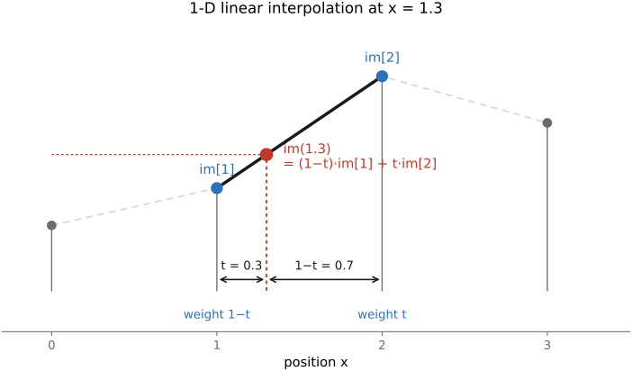
Drop to one dimension, where the idea is cleanest. An image row is a 1-D array of values, and we want the value at $1.3$, between the samples at $1$ and $2$. The natural move is to blend the two neighbors in proportion to how close the query sits to each. At $1.3$ we are $0.3$ of the way from $1$ toward $2$, so
This is linear interpolation, and there is one detail that trips up everyone at first: the weights run opposite to the distances. The neighbor you are $0.3$ away from gets weight $0.7$, not $0.3$, because you want weight $1$ when you sit exactly on a sample and $0$ when you are a full step away. Say it back in words: take a weighted average of the two bracketing samples, weighting each by one minus the distance to it. Geometrically, the reconstructed signal is just the straight line connecting consecutive samples (Figure 6.5.3).
6.5.7 Bilinear, in 2-D⧉
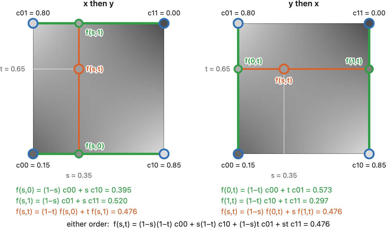
In two dimensions we now have four surrounding samples (the corners of the unit square the query falls inside) and two fractional coordinates to interpolate against. The clean construction is to do 1-D linear interpolation twice: first along $x$, then along $y$ (Figure 6.5.4). Blend the top pair of pixels horizontally to get one value, blend the bottom pair horizontally to get another, then blend those two results vertically with the $y$ fraction. The four corner weights come out as products of the $x$- and $y$-blend factors, which is exactly why this is bilinear: linear in each axis, but their product, not a single plane through all four points.
That last point is a real subtlety. Four arbitrary corner values do not in general lie on a flat plane, so a "purely linear" 2-D surface through all four simply does not exist. Bilinear sidesteps this by being linear separately in each direction (the product of two tents), which is well-defined and cheap. The resulting surface is doubly ruled: dead straight along every horizontal and every vertical line, yet curved overall, twisting into a saddle when the four corners disagree (Figure 6.5.5). The only way to get a truly planar piecewise-linear reconstruction is to triangulate: cut each square into two triangles and interpolate within each, since three corners do fix a plane.
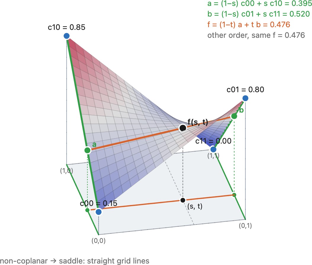
The next stage of Figure 6.5.1 applies bilinear interpolation to the whole image.
If you do triangulate, you must choose which diagonal to cut each square along, and the two choices differ near edges. A naive splitter always cuts the same way, secretly preferring one diagonal and producing a faint directional bias. The smarter trick picks, per square, the diagonal joining the two most similar corner values, cutting along an edge rather than across it, so a sharp boundary isn't smeared. Bilinear's quiet advantage is that it has no diagonal to choose: it needs no branch and favors no direction.
Choosing the diagonal of each cell from the data is data-dependent triangulation, introduced for image reconstruction by Yu, Morse and Sederberg (2001); the per-cell rule of the sidebar is the pixel-level version of Su and Willis (2004), and the fifth stage of Figure 6.5.1 runs it after bilinear.
Show that interpolating $y$ first, then $x$ gives exactly the same result as $x$ first, then $y$. (Write both as weighted sums of the four corners and compare the coefficients, the order of the two separable passes does not matter.)
Putting the two halves together (the inverse-mapping loop and the bilinear sample) gives the whole upsampler. Loop over output pixels, send each back through $f^{-1}$ to a fractional input location, split that into its integer cell and fractional offsets, and blend the four corners:
for each output pixel (x, y):
    (u, v) = f⁻¹(x, y)                  # fractional input location
    x0, y0 = floor(u), floor(v)
    s, t = u - x0, v - y0               # fractional offsets in [0, 1)
    top = (1 - s)·I[x0, y0]   + s·I[x0+1, y0]
    bot = (1 - s)·I[x0, y0+1] + s·I[x0+1, y0+1]
    out[x, y] = (1 - t)·top + t·bot     # blend the two rows vertically
Read it back: the two horizontal blends collapse the top and bottom edges of the cell, and the final vertical blend combines them: 1-D linear interpolation done twice. Bilinear is the workhorse default: cheap, no blocky tiles, smooth enough for most resizing, and the reconstruction you get for free from a graphics-hardware texture lookup (Figure 6.4.16, bilinear panel). But it has a ceiling. The reconstructed surface has creases (it is only continuous, not smooth, kinking at every sample) and on a strong upscale it reads a touch soft. To push past it we need to look at more than four neighbors, and the "interpolate between neighbors" story does not generalize gracefully. We need a better lens, but first a word on what any of this costs.
For axis-aligned resizing, the horizontal coordinates and weights repeat across rows, and the vertical weights repeat across columns. Precompute both weight tables and apply two 1-D passes. A rational scale has repeating fractional phases away from boundaries. An arbitrary warp does not generally factor into two image-wide passes, even when its local kernel is separable. Normalize weights according to the selected boundary rule; dropping out-of-bounds taps and renormalizing is one rule, not a substitute for choosing one.
6.5.8 The convolution perspective⧉
Here is the more general formulation. So far we have described reconstruction as interpolating between neighbors. That picture is fine for linear interpolation and for upsampling, but it has two failings: it does not extend cleanly to fancier reconstructions, and it does not extend to downsampling at all. Since this whole chapter is fundamentally about (re)sampling, the Fourier-flavored view from Chapter 6.4, Sampling, downsampling, and aliasing has much better insight to offer. In practice that view means one thing: reconstruction is convolution.
Concretely, the output value at a fractional location is a weighted sum of nearby input pixels, with the weights read off a smooth analytical kernel $k$ centered at the desired (non-integer) location. Slide a continuous kernel so its center sits exactly on the query point $f^{-1}(x,y)$, evaluate the kernel at each surrounding integer input pixel to get that pixel's weight, and sum. The general resampling formula is
summing over input pixels $x'$ in the neighborhood, the kernel evaluated at the offset between the query and each pixel. In words: to find an output pixel, inverse-transform it to a fractional input location, drop a smooth kernel centered there, and accumulate kernel-weight times pixel-value over the nearby samples. It is convolution, but where convolution in the earlier chapter lived purely on the integer grid, here the kernel is a continuous function we can evaluate at any fractional offset (ask for $k(-0.7)$ and it answers), because the center is non-integer.
The resampler needs weights for fractional offsets. A formula for a real-valued argument supplies them, as do a lookup table or a bank of filters for quantized fractional phases. A list of integer-offset convolution taps alone does not specify interpolation between taps. Nearest neighbor’s box kernel is discontinuous, so continuity is not a requirement.
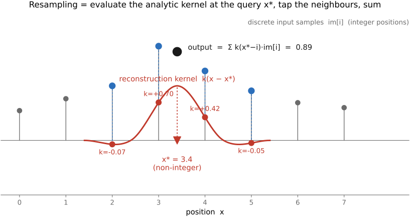
Bilinear is already a special case. The linear-interpolation weights $0.7$ and $0.3$ are exactly the values of a triangular (tent) kernel, one that is $1$ at its center and falls linearly to $0$ one sample away on each side, evaluated at the offsets to the two neighbors. So "interpolate linearly" and "convolve with a tent" are the same operation, seen two ways. Nearest neighbor is the same story with a box kernel (a flat $1$ over a one-pixel window). Once reconstruction is "convolve with a kernel," choosing a better reconstruction is just choosing a better kernel.
Figure 6.5.7 draws these kernels as 2-D kernels $k(x)\,k(y)$, each with its profile, an upsampling made with it, and its Fourier transform, starting with the box and the tent.
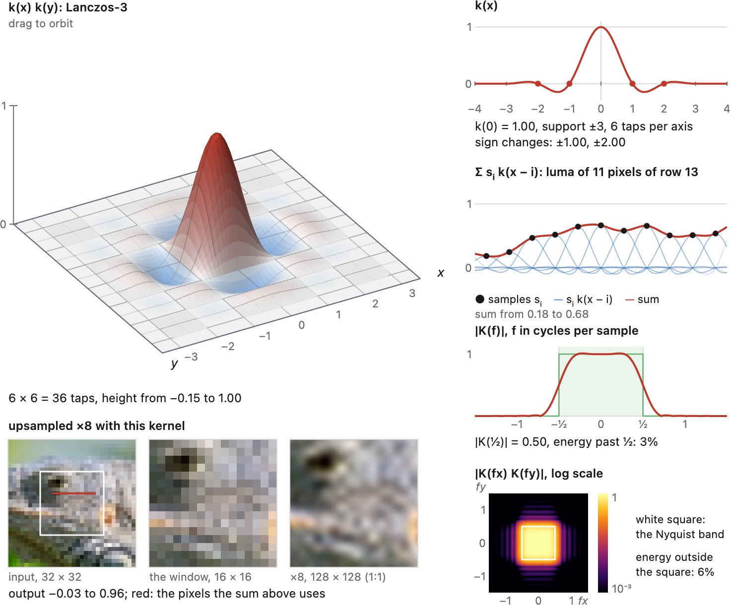
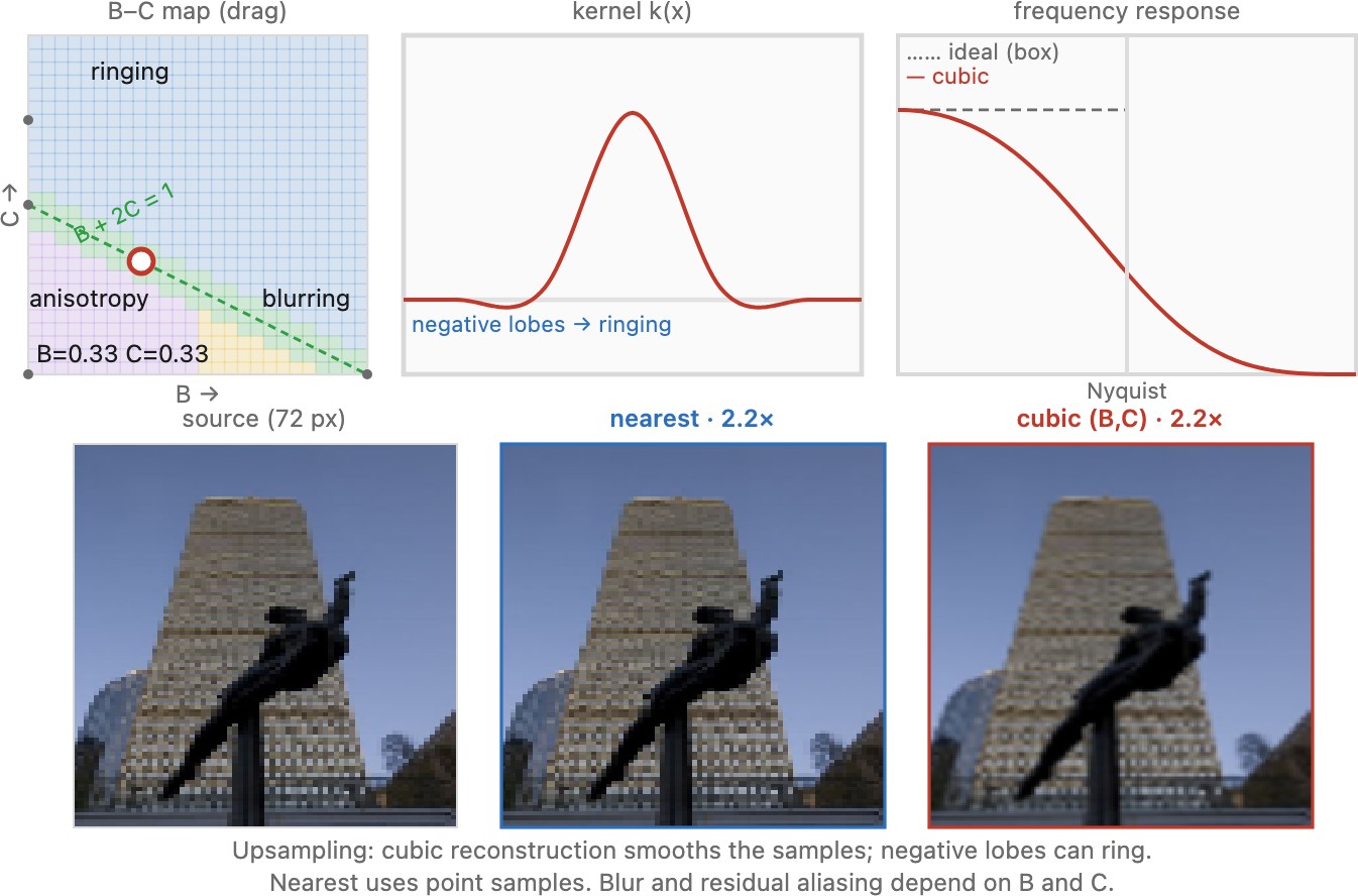
The box and the tent are the crudest kernels. Better ones, the Mitchell–Netravali cubics $k_{BC}$ and the Lanczos windowed sinc, are developed as approximations of the ideal sinc in Chapter 6.4, Sampling, downsampling, and aliasing, where they first serve as prefilters for downsampling. As reconstruction kernels they upsample with less blur than the tent and without the box's blocks, at the price of some overshoot near edges.
The third stage of Figure 6.5.7 draws any member of the family in 2-D, with its Fourier transform.
The sixth stage of Figure 6.5.1 upsamples with any member of this family.
Its last stage swaps the cubic for the Lanczos kernel, with order $a$ from 2 to 4.
The last stage of Figure 6.5.7 draws the Lanczos kernel the same way, for orders 2 to 4.
6.5.9 The full signal-processing view: sample, reconstruct, prefilter, resample⧉
The kernels above are one part of a pipeline that explains every resampler in this chapter. We write it in one dimension, with input samples $I(j)$ at the integers and output samples at a spacing $q$ measured in input pixels, so $q>1$ shrinks the image and $q<1$ enlarges it. Two dimensions repeat it along each axis, and a general warp replaces the output position $mq$ by $f^{-1}$ of the output pixel.
The sampled representation. The input is a list of numbers, not a function. We represent it as a train of impulses, $I_\delta(x)=\sum_j I(j)\,\delta(x-j)$. In the frequency domain, sampling at unit spacing makes the spectrum periodic, $\hat I_\delta(u)=\sum_n \hat I(u-n)$: copies of the spectrum of the underlying continuous image, one every cycle per pixel (Chapter 6.4, Sampling, downsampling, and aliasing). The band $|u|<\tfrac12$ holds the information; the copies are what sampling added.
Figure 6.5.8 follows these steps on one row of an image, one column per step, each signal above its spectrum.
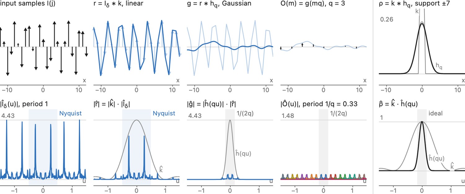
Reconstruction. Convolving the impulses with a kernel $k$ gives a continuous image, $r(x)=\sum_j I(j)\,k(x-j)$, the formula of the previous section. In frequency the convolution becomes a product, $\hat r(u)=\hat k(u)\,\hat I_\delta(u)$. The ideal $k$ is the sinc, whose transform keeps the central copy and removes the others. A practical kernel does both jobs imperfectly: it attenuates the central copy near $u=\tfrac12$, which blurs, and it keeps part of the neighboring copies, which shows as blocks or staircases. This is imaging, the reconstruction counterpart of aliasing.
The second stage of Figure 6.5.8 adds the reconstruction.
Prefiltering. If the output grid is coarser than the input, $r$ still holds frequencies up to half a cycle per input pixel, more than the output can represent. A low-pass filter scaled to the output spacing, $h_q(x)=\tfrac1q\,h(x/q)$, removes them: $g=r*h_q$, and $\hat g(u)=\hat h(qu)\,\hat r(u)$, ideally a box that keeps $|u|<1/(2q)$. When enlarging, $q<1$ and that band is wider than what reconstruction already left, so the prefilter has nothing to do.
The third stage adds the prefilter.
Sampling on the new grid. The output is $O(m)=g(mq)$. Sampling at spacing $q$ makes the output spectrum periodic again, with copies every $1/q$; whatever $\hat g$ still holds beyond $1/(2q)$ folds back into the band as aliasing.
The fourth stage samples the new grid.
Reconstruction and prefiltering are both convolutions, so they combine into one kernel, $\rho=k*h_q$, and the whole pipeline collapses into a single weighted sum per output pixel:
When enlarging, $\rho$ is essentially the reconstruction kernel $k$, which keeps its width in input pixels. When shrinking, it is essentially the prefilter $h_q$, whose width grows with the reduction. This is the scaled kernel of the next section, whose normalized formula is this sum with $\rho$ replaced by the stretched kernel (Figure 6.5.9). Figure 6.4.9 shows the same steps for the first sampling of a continuous signal.
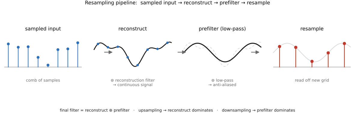
The last stage of Figure 6.5.8 draws $\rho$ beside the pipeline.
6.5.10 Upsampling vs. downsampling: scale the kernel⧉
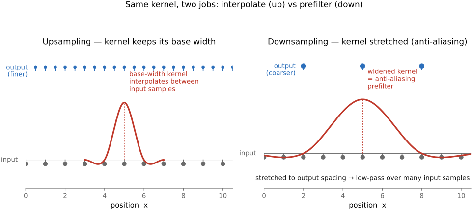
We have promised twice that downsampling reuses the same machinery; now we cash it in. Whether you scale up or down, you run the same convolution with the same family of kernels. The only thing that changes is how you scale the kernel.
When upsampling, the kernel keeps a fixed footprint in the input image (about four pixels wide for bicubic, however much you enlarge) because the input samples are already dense enough; you are just reading between them. So for upsampling the kernel width in input space is constant (a useful corollary: clamp the kernel's scale factor at $1$, never narrower).
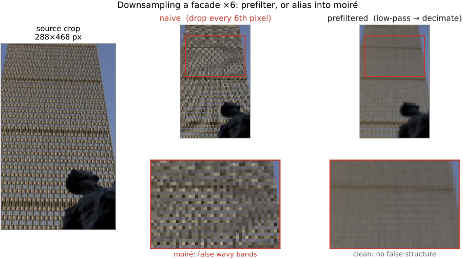
Downsampling is the harder case, and not by a little. Pick one input pixel per output pixel (nearest neighbor, no blur) and you get aliasing: a fine texture turns into bold, wrong, low-frequency moiré (a brick wall or a striped shirt shot from far away dissolving into wide phantom bands; Figure 6.5.13). This is not a cosmetic glitch but the wagon-wheel / Prudential-tower effect from Chapter 6.4, Sampling, downsampling, and aliasing: detail finer than the output grid can represent does not vanish, it folds down and masquerades as coarse structure.
Widen the filter in proportion to the reduction. In one dimension, let $q=W_{\mathrm{in}}/W_{\mathrm{out}}$ and $a_s=\max(1,q)$. A practical normalized resampler uses
The source coordinate is $u$. The sum covers the stretched kernel’s support. A fivefold reduction stretches a four-sample cubic support to twenty input samples, not five. Normalization preserves a constant image when the denominator is nonzero. Finite support still permits residual aliasing. How much depends on the kernel as well as its width. A box as wide as the reduction, the plain average of each block, is the most common prefilter and one of the leakiest: the sidelobes of its transform pass a fine periodic texture. Shrinking the facade of Figure 6.5.8 threefold, 88% of the energy that ends up in the output band is aliased with a box prefilter, against 9% with a Gaussian and 2% with Lanczos-3 (stage prefilter).
Pixel-center conventions also matter. With centers at integer indices and image edges at half-integers, use $u=(x+1/2)W_{\mathrm{in}}/W_{\mathrm{out}}-1/2$. This differs from aligning the first and last centers. Choose one convention and use it consistently when composing transforms.
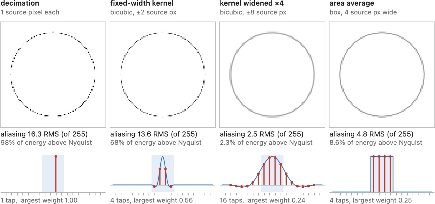
Not every resize function widens it. Parmar et al. found that several widely used libraries reduce an image with a kernel of fixed width by default; Figure 6.5.12 puts that behavior beside the alternatives and traces the aliasing to the kernel.
The effect is ugliest on real, regular structure: the rows of windows on a glass facade, shrunk for a thumbnail, break into sweeping moiré if you decimate without prefiltering (Figure 6.5.13).
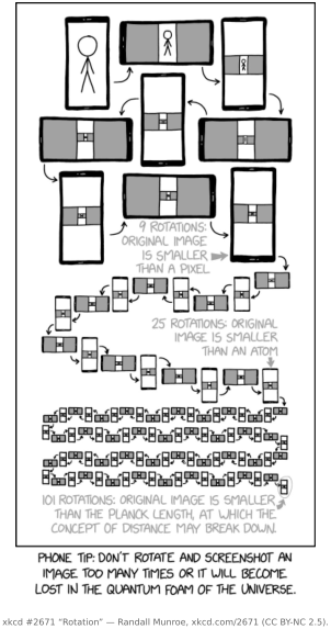
Rotate an image through a full turn in $N$ equal steps, each resampling the previous result. Compare it with one resampling using the composed transform. The repeated version accumulates interpolation error even though the net geometry is identity. Sharper kernels can retain more detail but may also amplify ringing. No finite resampler guarantees that hundreds of rotations recover the original. Evaluate only the region whose source support remains valid throughout.
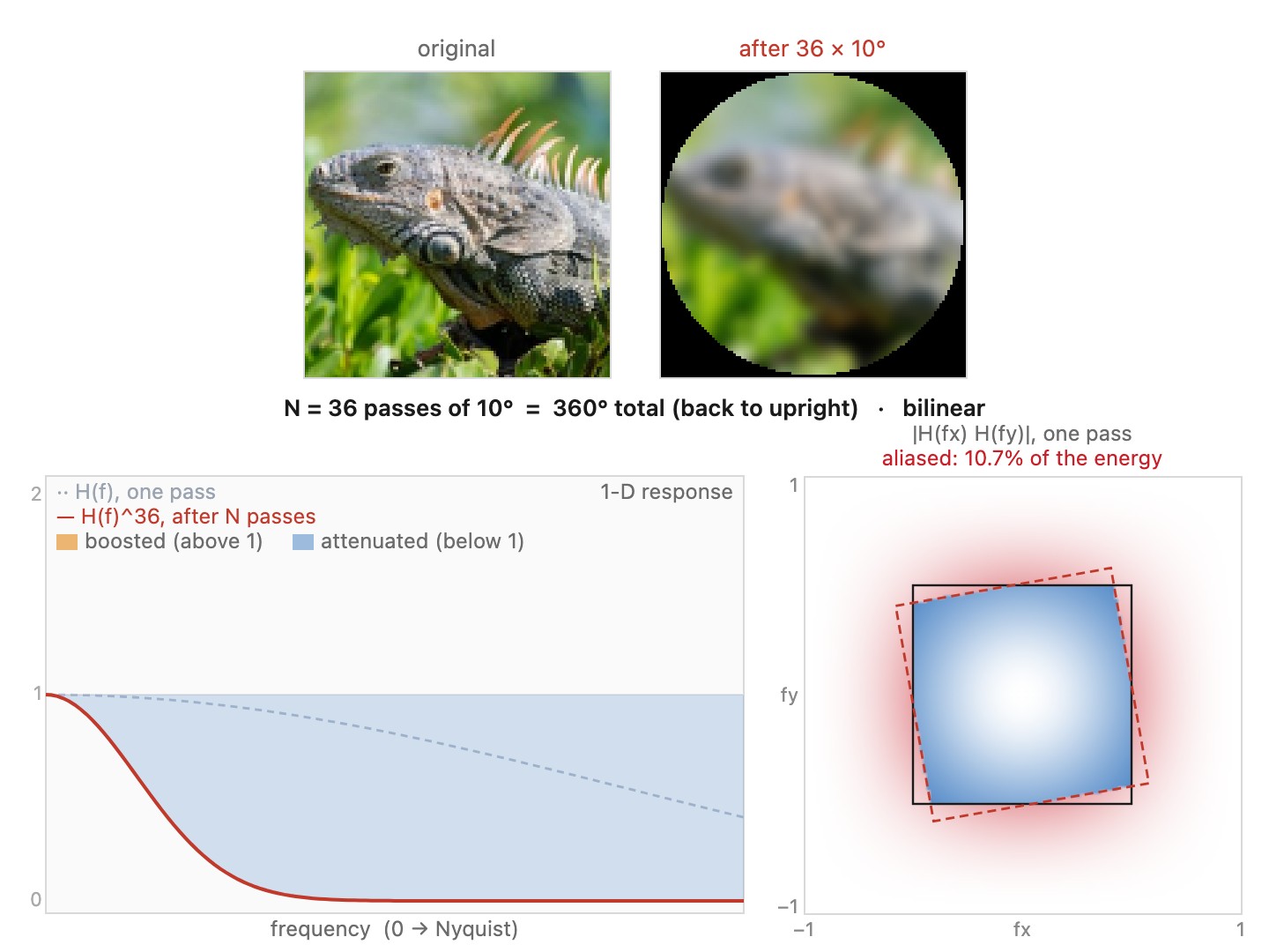
Repeated resampling accumulates blur, ringing, and sampling error. For repeated fixed convolution the frequency response is exactly $H^N$; for rotations it is only an illustration because the grid and effective filter change at each pass. Compose geometric transforms and resample the original once.
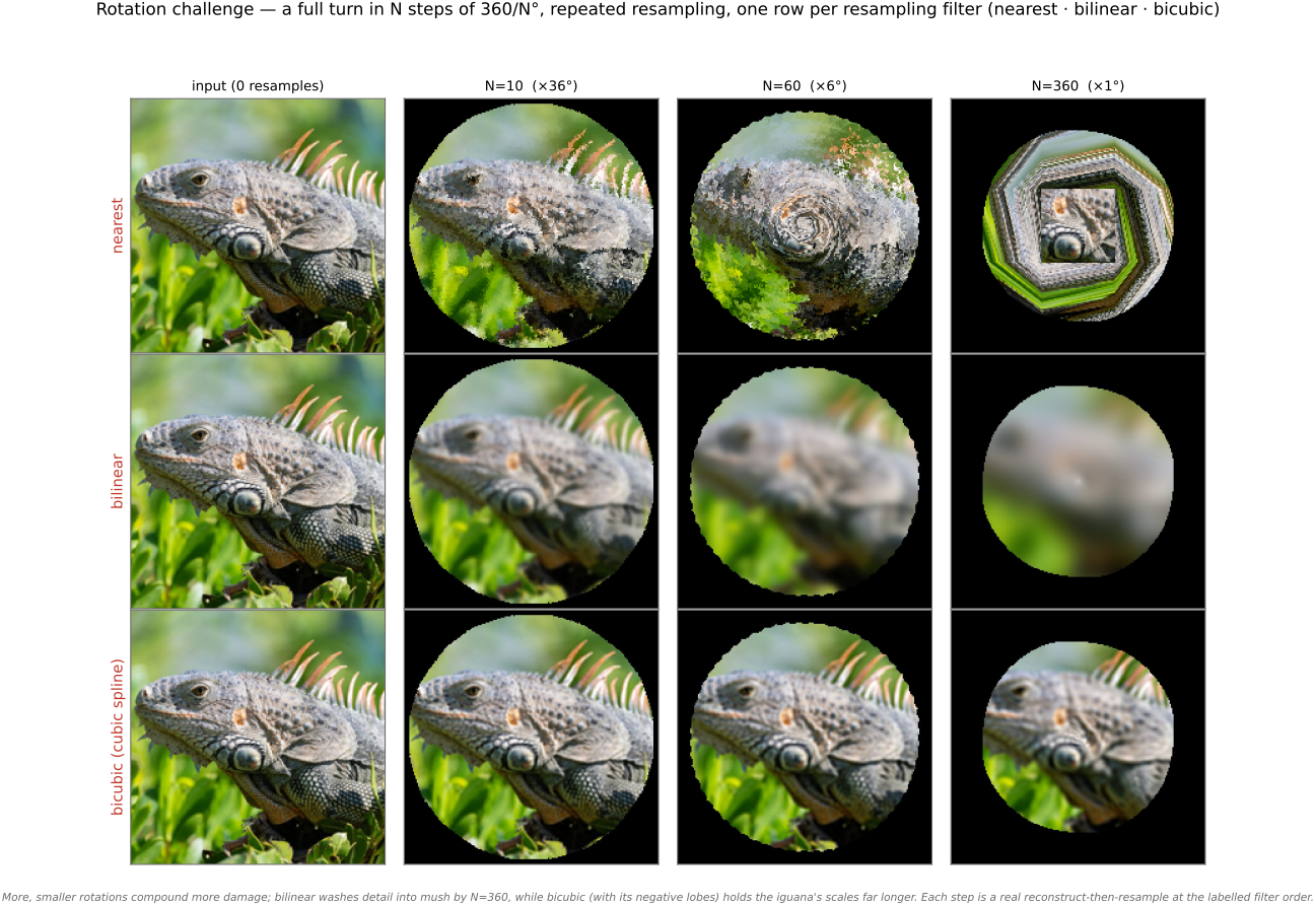
Run the same experiment yourself in the interactive version below: one image, your choice of total angle and step size (the total is rounded to a whole number of steps), and any of five filters, and when you pick bicubic, the same $(B, C)$ handle from above to dial the cubic between blur and ring.
For a far deeper practical treatment of resampling filters, their windows, and the subtle quality differences between them, Nicolas Robidoux's analysis for ImageMagick is the reference worth reading (<https://usage.imagemagick.org/filter/nicolas/>); it is the kind of care that separates a library taking resampling seriously from one that ships a default and hopes.
6.5.11 Prefiltering when the transform isn't a clean scale⧉
An affine map sends a square output footprint to a parallelogram in the input. Elliptical weighted average (EWA) filtering approximates the footprint with an ellipse. Its shape can be obtained from the Jacobian $J$ of the inverse map: a circular footprint with covariance $C$ maps locally to covariance $JCJ^\top$. An affine map has the same Jacobian everywhere; a perspective or nonlinear map generally does not. A pure rotation changes orientation without changing area or introducing unequal axis scales.
Mipmaps choose among prefiltered resolutions cheaply; EWA accounts more closely for directional compression. Both approximate the combined reconstruction and output filtering. Chapter 11.2, Antialiasing for complex transforms develops the footprint model.
A resample is a weighted average of neighboring pixels, and an average is only physically meaningful on values proportional to light, i.e. linear radiance. Most image files are gamma-encoded (sRGB), and averaging the encoded values is wrong: the encoding is concave, so the mean of two encoded values is darker than the encoding of their mean. The visible symptom is the classic "gamma-incorrect" darkening on downsampling and on antialiased edges: thin bright features on dark backgrounds lose energy, and mip-mapped textures go muddy. The fix is the standard ISP discipline (Chapter 45.15, Rendering a raw DNG): decode to linear, resample, re-encode, once, around the whole pass. Log space is a third option, but a perceptual / dynamic-range one rather than a physically correct one: averaging in log is a geometric mean that down-weights a few very bright pixels and can look better on extreme-HDR content, but for ordinary resampling linear is the correct default and gamma is the trap.
This matters on a receding surface. One output pixel may cover little source extent in one direction and a long strip in the other. Choosing one isotropic mipmap level large enough for the strip can erase useful detail across it; choosing a finer level can leave aliasing along it. An anisotropic footprint spends its averaging in the compressed direction. Ripmaps, multiple texture probes and EWA make different approximations to this same coverage problem, developed in Chapter 11.2, Antialiasing for complex transforms.
6.5.12 Resampling and encoding⧉
To approximate spatial integration of light, decode the transfer curve, filter in linear light, then encode again (Chapter 4.3, Encoding: linear, gamma or log). With nonnegative normalized weights, sRGB decoding is convex, so decoding the average code value gives no more light than averaging decoded values. Signed kernels such as Lanczos do not obey this inequality.
An equal mixture of black and white illustrates the size of the error: their sRGB codes average to 0.5, which decodes to about 0.214 linear light; their light average is 0.5, encoded as about 0.735. Low-contrast regions have smaller discrepancies. A deliberately chosen perceptual-space operation is possible, but it is a different operation from integrating light.
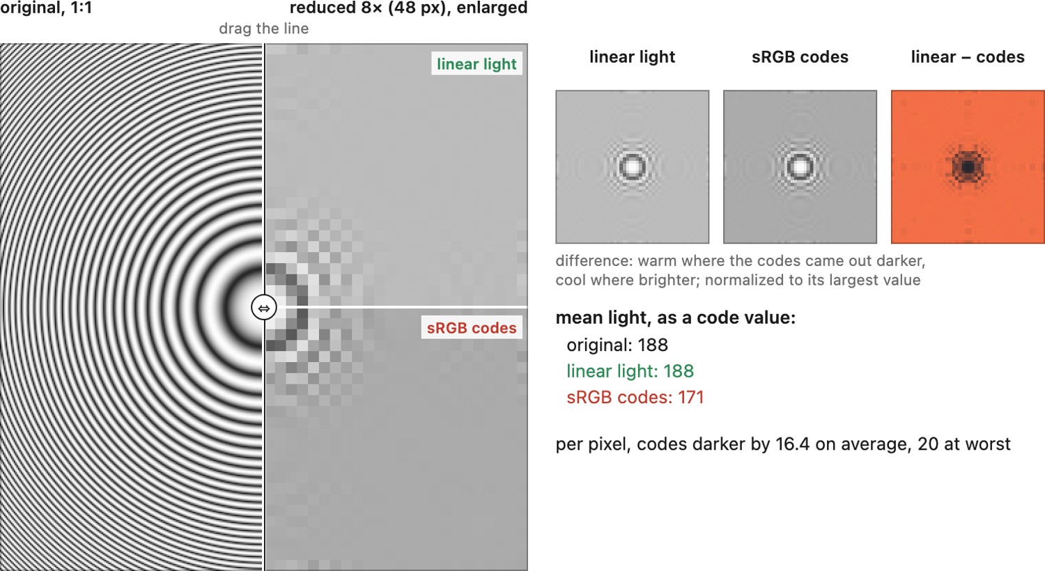
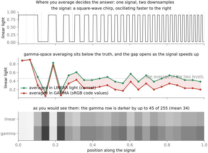
Do not infer the processing domain from a library or filter name. Set it explicitly and check with a black-and-white pattern. For transparent images, filter premultiplied linear RGB and alpha together, then unpremultiply where alpha is nonzero. Otherwise arbitrary colors in transparent pixels can bleed into visible edges.
6.5.13 Beyond Nyquist-limited reconstruction⧉
The fixed kernels above are linear for fixed geometry and weights, but separable kernels are generally not isotropic. They cannot determine arbitrary detail missing from the samples. Content-dependent reconstruction uses extra assumptions, such as locally smooth regions separated by edges.
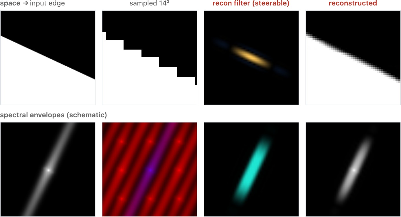
But, exactly as with deblurring, we are rarely without further assumptions. Natural images are not arbitrary signals: they occupy a thin, structured manifold (the natural-image prior of Chapter 7.1, Imaging as Bayesian inference with probabilistic priors), and we can exploit those regularities to beat the worst case. One regularity matters here especially: images are locally anisotropic. Near an edge there is content in essentially one direction (across the edge) and almost none along it. That has a precise Fourier consequence: the local spectrum is concentrated on a line (or a narrow wedge), so when sampling replicates the spectrum, the alias copies land in only part of the Fourier plane, leaving large regions where we know no alias can be.
If the local edge orientation is known, an elongated filter can average along the edge while preserving variation across it. This can improve reconstruction under that scene model. It does not separate every overlap of spectral replicas: some edge orientations and textures remain ambiguous. Estimating orientation from the same aliased data introduces another possible error. The complete adaptive procedure is generally nonlinear even though filtering with frozen weights is linear.
This steered, content-adaptive strategy is the workhorse of demosaicking and of older super-resolution. Many demosaicking methods follow exactly this two-step recipe: first analyze the local orientation and pattern (is there an edge here, and which way does it run?), then steer a reconstruction filter to interpolate along the edge rather than across it, which is what keeps demosaicked edges from breaking into the colored zipper artifacts a naive isotropic interpolation produces.
The modern version of the same idea drops the hand-built orientation analysis and instead learns the regularities of natural images directly (and learns how to reconstruct them) from data. That is where super-resolution and demosaicking have largely gone (and where this book picks them up again in the learning chapters): the prior is no longer "images are locally oriented," written by hand, but a model trained to know what the high-resolution image probably was.
Finally, there is a second kind of luck, and it changes things entirely. Sometimes we are not reconstructing blind: we already hold a high-resolution image that we know is correlated with the very quantity we are trying to recover. This is the common situation in colorization and in local image adjustments, where the thing being upsampled (the chrominance, or a per-pixel correction) is often correlated with the high-resolution guide’s edges. Two families of methods turn that correlation into resolution. Cross / joint bilateral filtering reads its edge-stopping weights from the high-resolution guide while it filters the low-resolution quantity, so the upsampled result inherits the guide's edges (forward ref: Chapter 10.1, Bilateral filtering §cross/joint, and Chapter 10.6, Guided image filtering). Or we can pose an optimization that asks the output to differ between two neighboring pixels only as much as the input does, encouraging the correlations among output pixels to match those among input pixels (forward ref: Chapter 10.3, Edge-preserving optimization — colorization and Chapter 10.5, Matting Laplacian). Either way the high-resolution guide supplies candidate structure; mismatched edges can transfer texture or create false boundaries, a recurring theme of the chapters in Edges matter.
6.5.14 Practical implementation choices⧉
For a reproducible resize, specify the coordinate convention, kernel and scale, boundary extension, processing domain, and alpha treatment. Check that a constant image stays constant, an identity transform reproduces samples for an interpolating kernel, and a fine pattern is adequately filtered during reduction. Compose successive transforms before sampling.
Recap: big lessons of this chapter
Loop over output pixels and pull back through $f^{-1}$ to find where each one reads from. Gathering fills every output exactly once; scattering pushes input pixels forward and leaves holes whose shape depends on the transform, a lattice of gaps under a scale and tilted slivers under a rotation. The same reflex governs warping, morphing, texture mapping, and flow-based reprojection later. Scattering earns its place only when the forward map is the thing you actually have, as in splatting a point cloud, and then it needs an explicit accumulation and normalization pass.
Repeated resampling accumulates blur, ringing, and sampling error. For repeated fixed convolution the frequency response is exactly $H^N$; for rotations it is only an illustration because the grid and effective filter change at each pass. Compose geometric transforms and resample the original once.