6.2 Convolution⧉
PS2 implements box/Gaussian blur, gradients, sharpening, and the bilateral filter. → Chapter 1.5, Problem sets (appendix).
A blur softens an edge by mixing neighboring values. A derivative measures their differences, and a sharpener adds some of those differences back. All three can use one table of weights applied throughout the image, a convolution kernel.
Blurring is useful before downsampling, for noise reduction, and for building image pyramids. It also models some optical degradation. A single kernel is appropriate only when the point spread is the same across the region being modeled; depth changes and camera motion often require a more general operator.
Sharpening increases local contrast. It can make surviving detail easier to see, but it is not generally the inverse of the blur that formed an image.
6.2.1 Convolution as a weighted sum of neighboring pixels⧉
A kernel assigns a weight to each displacement between an input and an output sample. Nonnegative weights summing to one form a local average. Derivative and sharpening kernels can have negative weights, so convolution is more general than averaging.
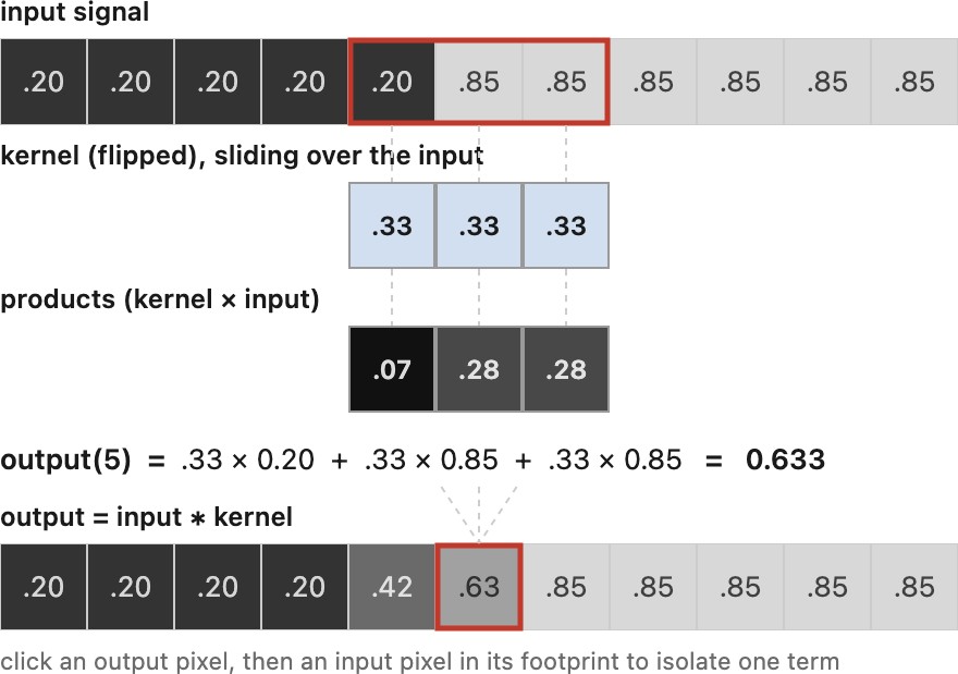
It is easiest to see in one dimension first (Figure 6.2.1), where the whole operation is a 3-tap kernel sliding along a row of pixels: each output pixel is the weighted sum of the three input pixels under the kernel, and nothing more.
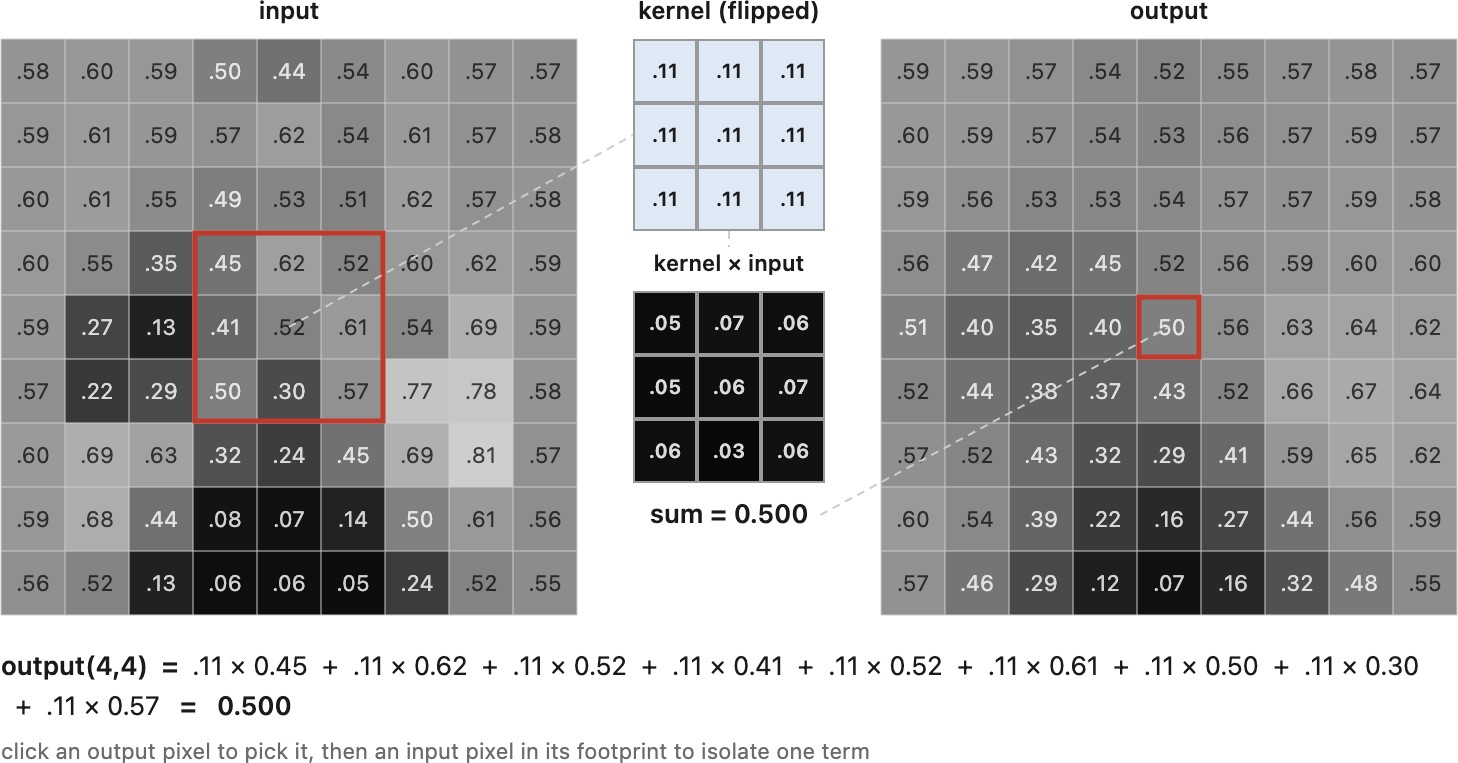
The two-dimensional case is the same thing with a small grid of weights instead of a row (Figure 6.2.2).
Two properties of this scheme are important. First, it is linear: each output pixel is a weighted sum of input values with fixed weights, so scaling the input scales the output, and adding two images adds their outputs. Second, it is shift-invariant: the same kernel applies at every pixel, so the operation does not care where in the image you are. Formally, writing $S_d$ for a shift by $d$ pixels, a shift-invariant operation commutes with shifting, $F(S_d\,x) = S_d\,F(x)$: shift the input and the output just shifts to match. Such an operation is linear and shift-invariant (LSI). This characterization assumes an infinite grid or compatible periodic boundaries; finite-image extensions require separate attention below.
Both conditions are real constraints, and it helps to watch one break. A graduated neutral-density filter (the kind that darkens the sky at the top of the frame while leaving the foreground alone) multiplies each pixel by a factor that depends on its row, say $(1 - y/y_\max)$. That is still linear (scaling the input scales the output), but it is emphatically not shift-invariant: slide the image down and the darkening falls on different content. So it is a linear operation that is not a convolution. Convolution is the well-behaved special case where the rule is identical everywhere, and that uniformity is exactly what later lets the Fourier transform pry it open.
A convolution uses fixed weights that depend on displacement, not on image values or absolute position. On an infinite or periodic grid it is linear and commutes with shifts. The kernel can be small or span the image. Its support determines the work of direct filtering; finite boundaries determine where the shift-invariance model applies.
Defocus varies with scene depth, camera rotation produces position-dependent image motion, and aberrations can vary across the field. These effects may remain linear in scene intensity for fixed geometry while requiring different point-spread functions at different locations. A nearly constant PSF over a small patch can justify a local convolution. At depth or motion boundaries, occlusion can invalidate that approximation. Chapter 6.7, Image formation as a linear system treats general operators and Chapter 16.4, Blind deblurring develops camera-motion models.
A linear model lets us study which patterns a measurement preserves and which it attenuates. Physical mixing must act on linear-light values. Filtering encoded values is a different operation, even when the same arithmetic is used; Chapter 4.3, Encoding: linear, gamma or log explains the distinction.
The algorithm itself is a short loop. Zero the output, then for every output pixel, walk over the kernel, multiply each input neighbor by its weight, and accumulate:
for each output pixel (x, y):
    out[x, y] = 0
    for each kernel offset (x', y'):
        out[x, y] += in[x + x', y + y'] · g[-x', -y']
assuming the kernel's coordinates are centered on zero. The minus signs on the kernel coordinates are the flip: each input neighbor is multiplied not by the weight at its own offset but by the weight at the opposite one. That flip is exactly what separates convolution from correlation, and why it matters is the subject of the next section.
6.2.2 The flip: where-from vs. where-to⧉
The minus signs in the loop above, the kernel read at g[-x', -y'] rather than g[x', y'], are the flip. The textbook definition writes the same operation by subtracting the offset on the kernel:
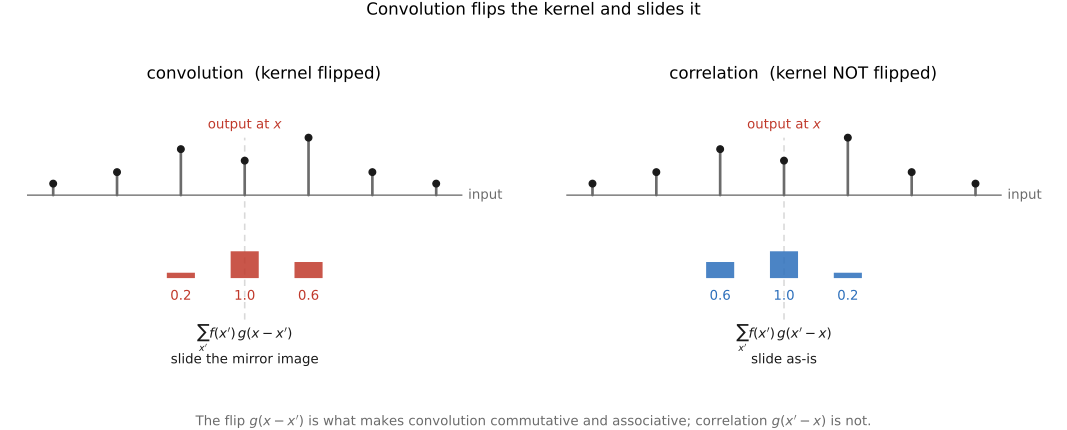
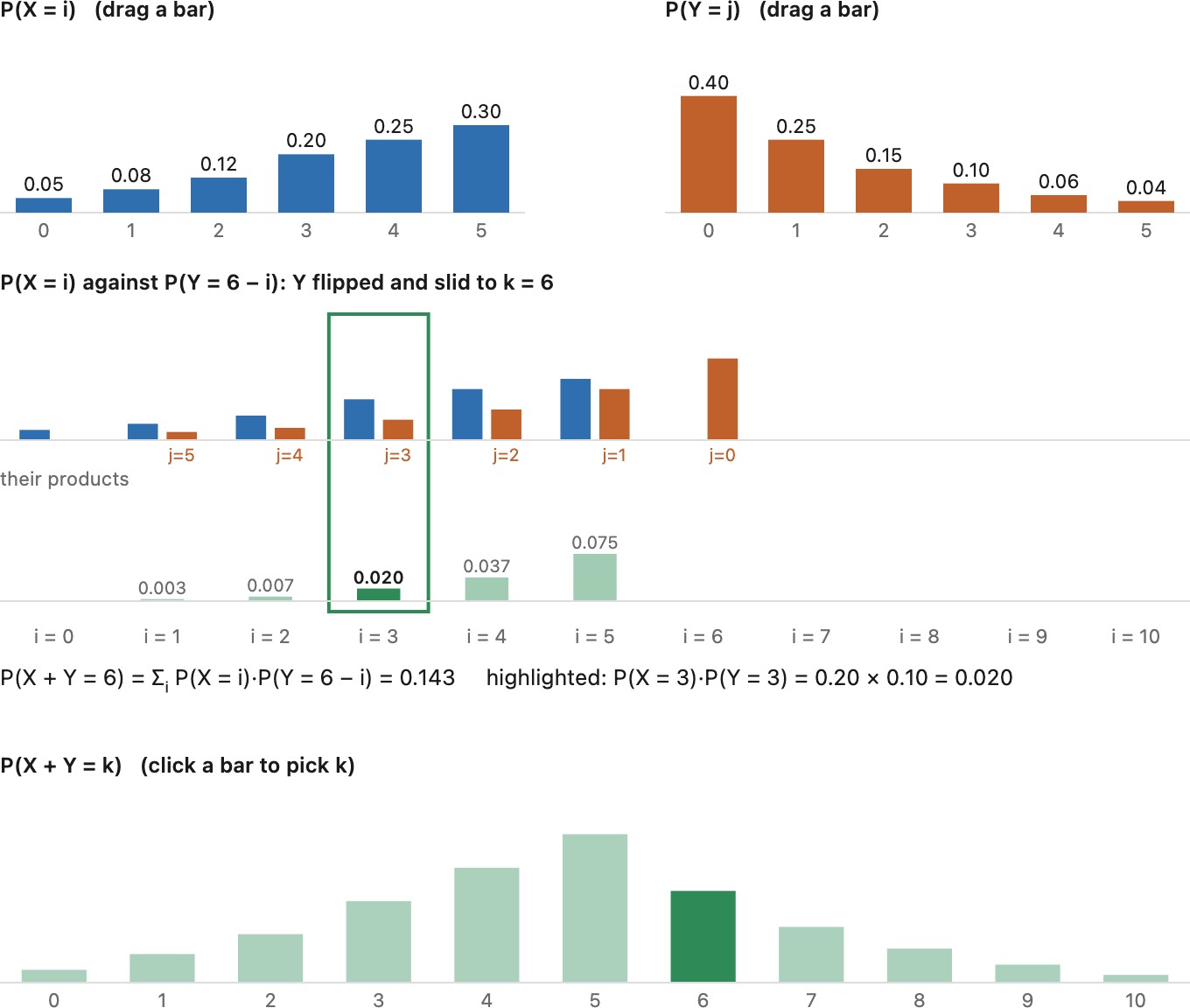
In words: to get the output at $x$, sum over all input positions $x'$, each weighted by the kernel evaluated at $x - x'$, the kernel is flipped (and slid) before it is multiplied in. Why the flip, and does it matter?
The flip is the difference between where light goes to and where light comes from. The physical, forward model says light at scene position $x$ lands, blurred, at sensor positions $x + x'$ for the offsets in the kernel; light spreads outward. But when we compute the output at a fixed pixel $x$, we are asking the backward question: which input pixels contributed here? The answer is the ones at $x - x'$. The minus sign is nothing but the bookkeeping of inverting "where-to" into "where-from."
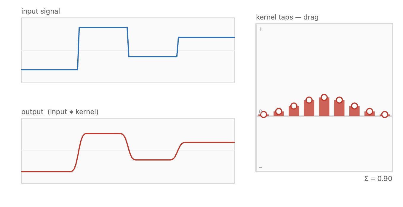
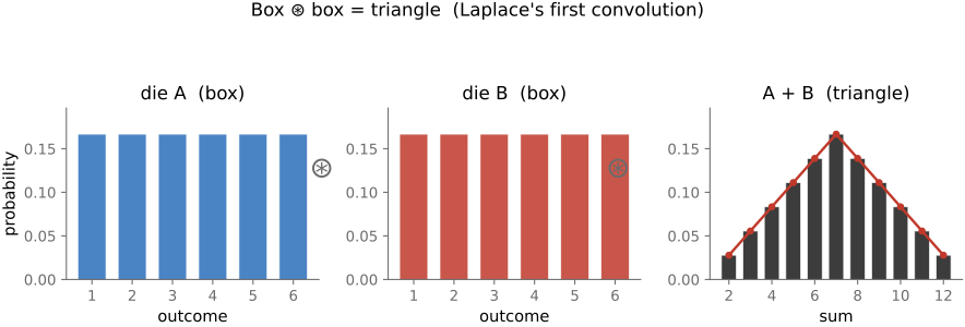
If $X$ and $Y$ are independent with known distributions, the distribution of $X + Y$ is their convolution, and the flip falls out for free. To ask "how likely is $X + Y = x$?", enumerate the ways it can happen: $X = x'$ paired with $Y = x - x'$, for every $x'$. The second variable is forced to be the sum minus the first, and you add up the products of probabilities over all $x'$. That $x - x'$ is exactly the convolution flip, here not a convention but a logical necessity. The cleanest instance is two dice: each die is a flat distribution over 1–6 (a one-dimensional box), and the distribution of the total is that box convolved with itself, a triangle peaking at 7 (Figure 6.2.5). This is why, throwing two dice, a sum of 7 is much more likely than a 12: there are six ways to roll a 7 (1+6, 2+5, 3+4, 4+3, 5+2, 6+1) but only one way to roll a 12 (6+6), so a 7 comes up six times as often, the middling totals win because there are simply more ways to reach them. A box convolved with a box is a triangle; the box returns in the blur zoo.
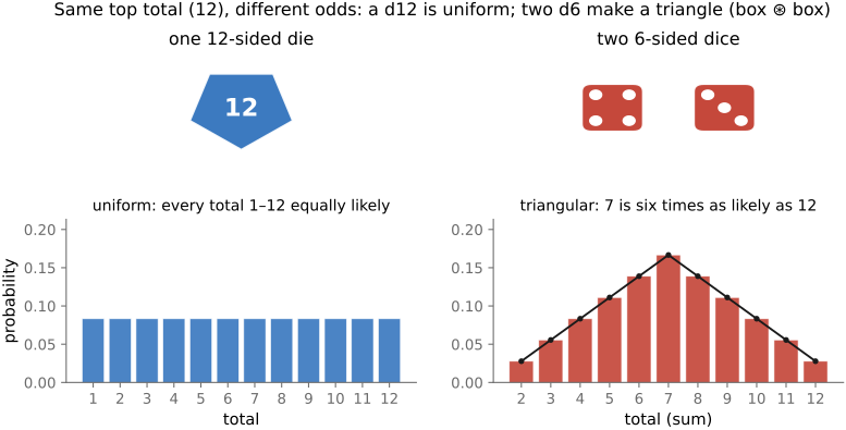
The same point is easy to miss with real dice. A single twelve-sided die and a pair of six-sided dice both top out at a total of twelve, yet they are nothing alike: the d12 is uniform (every total equally likely), while two d6 make a triangle, because their sum is a box convolved with a box (Figure 6.2.6).
For a symmetric kernel, convolution and real-valued correlation agree. For an asymmetric kernel, omitting the flip changes the operation; a derivative may reverse sign and a shift may reverse direction. Correlation is useful for matching a template against an image. State which convention the code uses rather than inferring it from a function name.
Test the convention with an asymmetric kernel rather than a Gaussian. A kernel with one nonzero tap displaced from its center should shift a single bright pixel in a predictable direction. Flipping the kernel reverses that direction. With a finite-difference kernel, the sign of a rising step distinguishes the two conventions. A symmetric blur cannot expose the mistake because it is unchanged by the flip. This is why a filter test suite needs a directional example even when the application mainly uses symmetric kernels.
A convolutional neural network does not flip. A "convolution" layer computes the correlation of its input with a learned kernel, which is what almost every deep-learning framework implements under that name. Nothing is lost by it: the kernel is fitted to data, so whichever orientation the layer needs, training finds it, and a flipped kernel is just as learnable as its mirror. The name is inherited from signal processing rather than earned. The distinction comes back in two places. One is at the boundary with classical code, where a kernel taken from a paper or from a library that does flip has to be flipped to match. The other is in the backward pass: the gradient of a correlation with respect to its input is a convolution, which is where the transposed convolution used in decoders and upsampling layers comes from. Chapter 7.3, Deep learning develops the layers themselves.
6.2.3 Convolution as a sum of translated images⧉
Everything so far has read convolution locally: fix an output pixel and gather a weighted sum of its neighbors. The same operation has a second, global reading. Instead of building the output one pixel at a time, build it one kernel tap at a time: each tap takes the whole input image, shifts it, scales it by the tap's weight, and adds it into the running total. Read this way, the output is a weighted sum of translated copies of the input, one copy per kernel tap.
The two readings are the very same double loop, only nested in the opposite order. Both zero the output, then run over every (output pixel, kernel offset) pair and add in[x + x', y + y'] · g[-x', -y'] each time. The one change is which for each line is the outer one; the body is identical. Coloring the output-pixel loop (blue) and the kernel-offset loop (red) makes the swap plain:
Local, the output-pixel loop on the outside:
out ← 0
for each output pixel (x, y):
    for each kernel offset (x', y'):
        out[x, y] += in[x + x', y + y'] · g[-x', -y']
Global, the kernel-offset loop on the outside:
out ← 0
for each kernel offset (x', y'):
    for each output pixel (x, y):
        out[x, y] += in[x + x', y + y'] · g[-x', -y']
In the local version the inner loop assembles one output pixel from all the taps; in the global version each pass of the outer loop adds one scaled, translated copy of the whole input, so the output grows as a sum of shifted images, $\text{out} = \sum_{x', y'} g[-x', -y']\,\cdot\,\text{shift}(\text{in},(x', y'))$. Same result, accounted from opposite ends. But the global reading buys three things the local one hides.
A fixed weighted sum of warped images is still linear in image intensity when the warps and interpolation weights are fixed. Pure camera rotation produces projective warps (homographies); roll alone is an in-plane rotation. Replacing shifts with these warps models motion that a single convolution cannot capture. Translation through a scene with varying depth also requires depth and visibility.
The global form also explains Fourier analysis: a complex exponential is multiplied by a scalar under each shift, so a weighted sum of shifts multiplies it by the weighted sum of those scalars. Chapter 6.3, Fourier develops this frequency response.
Translations commute on an infinite or periodic grid, so their weighted sum commutes with translation. Cropping or re-extending a finite image between operations can break this algebra.
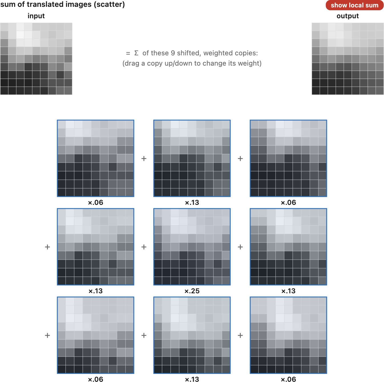
Convolution can be computed per output pixel or per kernel tap. In the first order we accumulate a neighborhood; in the second we accumulate shifted copies of the image. The result is the same. Replacing shifts with known warps gives other linear operators, but they need not share convolution’s commutativity or Fourier diagonalization.
6.2.4 Properties: the impulse, normalization, symmetry, commutativity⧉
A handful of properties make convolution pleasant to work with, and the slickest way to expose them is to feed the filter the simplest possible input: one bright pixel on a black background, the impulse $\delta$ (the discrete Dirac / Kronecker delta, one at the origin, zero everywhere else).
Convolve an impulse with a kernel and you get the kernel back, stamped at the impulse's location. The flip explains why: every output pixel asks "where did my light come from?", and the only nonzero input is the single bright pixel, so each output simply picks up the kernel weight that connects it to that pixel, tracing out the kernel. This output carries a name borrowed from optics: the point spread function (PSF), or impulse response. It is literally how the system spreads a single point of light, the very blob you saw around the streetlight. So the kernel, the impulse response, and the PSF are three names for one thing, with an immediate practical corollary: to discover what a filter does, feed it an impulse and read off the kernel. This is the single best debugging input for convolution code, and we will lean on it.
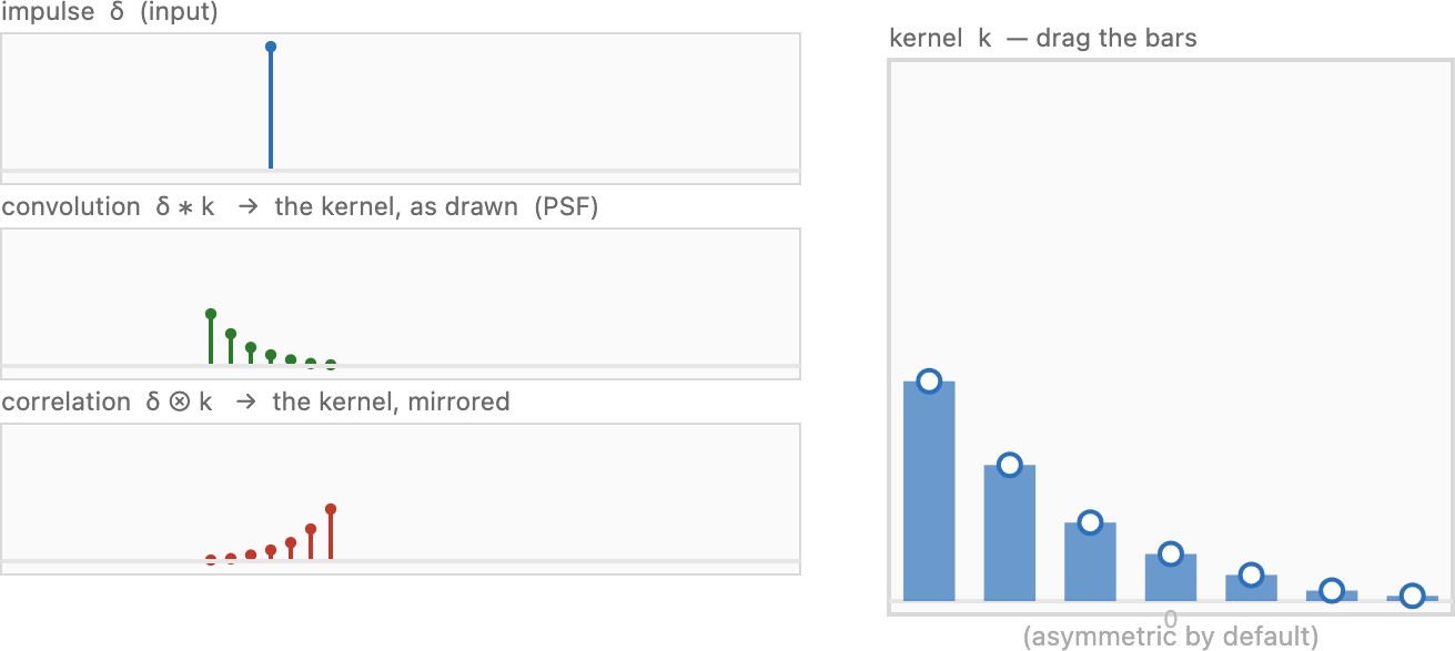
Convolve an interior impulse with an asymmetric kernel: the output should reproduce that kernel in its declared offset coordinates, not its flipped version. A constant tests unit-sum weights only where the boundary extension also preserves constants. A single nonzero off-center tap tests shift direction. A ramp tests derivative sign and scale, and an edge tests the step response. Start in one dimension and calculate a few outputs by hand. See Figure 6.2.9.
A straight step edge gives another measurement. Under locally shift-invariant blur, differentiating its edge-spread function gives the line-spread function, the PSF integrated along the edge direction. One edge orientation gives one projection, not the full two-dimensional PSF. A natural edge also includes its original softness, texture, noise, and earlier processing; controlled slanted-edge targets are used for quantitative MTF measurement.
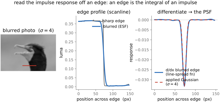
The identity element follows at once: convolving with the impulse leaves the image untouched, $I * \delta = I$, because reading "where-from" with a kernel that points only at yourself just copies you. The remaining properties:
- Normalization: weights summing to one preserve a constant signal when the boundary rule preserves that constant. This is not a guarantee that every finite crop preserves total energy. Derivative weights sum to zero; do not normalize them to one.
- Commutativity and associativity: on the full domain, $I*g=g*I$ and $(I*g)*h=I*(g*h)$. Consistent circular convolution has the same properties. Cropping and applying a fresh boundary extension after each pass can change the result.
- Linearity and shift-invariance together give the Fourier representation. Linearity alone does not make an operator diagonal in Fourier coordinates.
6.2.5 Nitty-gritty: finite images⧉
Two practical wrinkles before the kernels themselves.
First, the kernel must be centered. Our images place $(0, 0)$ at the top-left corner, but a blur kernel is naturally centered on the pixel it is computing, its weights run from $-r$ to $+r$ around the middle, where $r$ is the kernel radius, so the full size is $(2r+1) \times (2r+1)$. An off-by-one here shifts the whole image by a pixel; an impulse test catches it instantly, because the blob lands off-center.
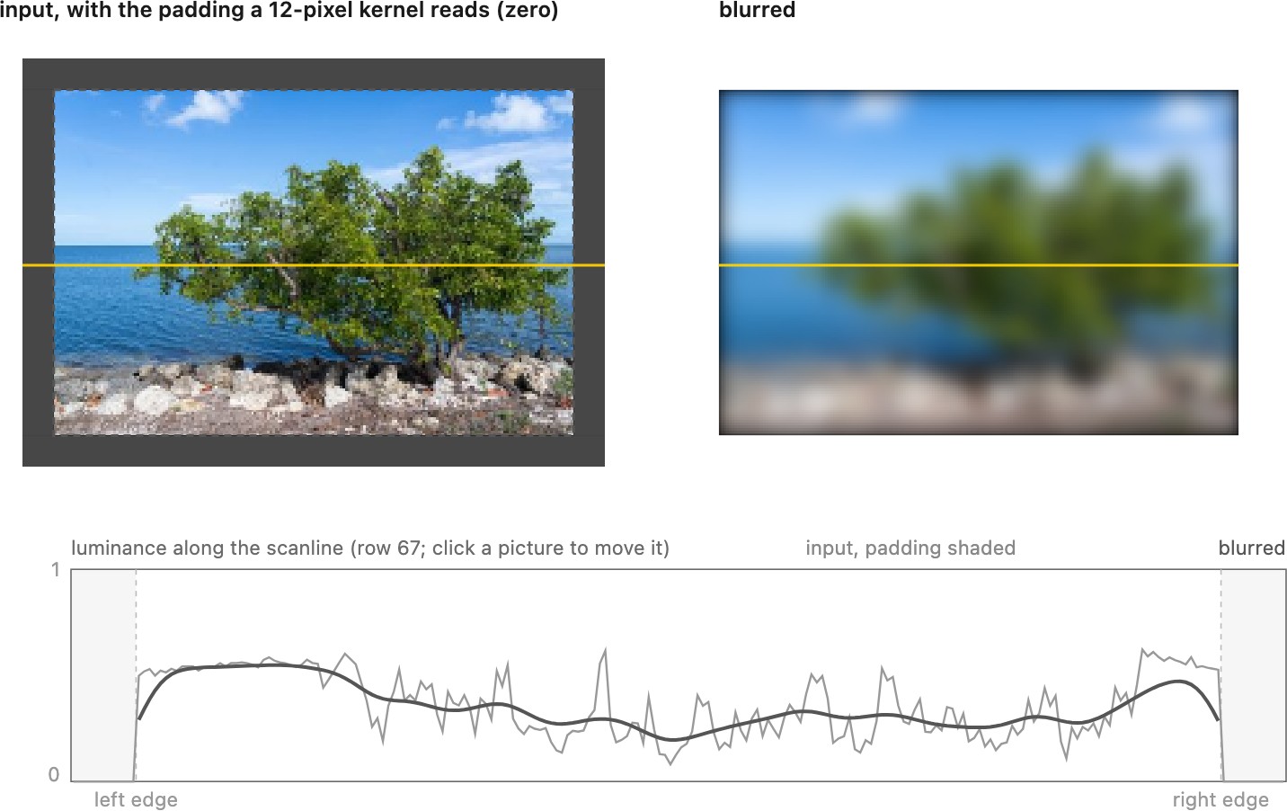
A finite image needs an extension rule: zero, repeated edge values, reflection, or periodic wrapping. Zero padding darkens a blurred border; reflection and clamping preserve constants but make different assumptions about missing content. Reflection conventions also differ in whether the edge sample is repeated. Use one declared convention in both the model and the implementation. Allocate a separate output buffer so earlier writes do not alter later inputs.
For a finite operator $A$, its transpose must reverse both filtering and boundary handling. A symmetric kernel does not by itself make a clamped or reflected implementation self-adjoint. This distinction matters when the filter appears inside an inverse solver.
6.2.6 A blur zoo⧉
With the mechanics settled, the only choice left is the kernel's shape. Two are worth knowing.
The box filter gives every sample in a $(2r+1)\times(2r+1)$ window weight $1/(2r+1)^2$. Its square footprint is not rotationally symmetric, and its frequency response has lobes and zeros. However, its nonnegative weights cannot create overshoot beyond the neighborhood’s range; a blurred step becomes a ramp, not a ringing edge. Running sums can make large box averages inexpensive.
The Gaussian is the workhorse. Its weights fall off smoothly with distance from the center, following the bell curve
where $r$ is the distance to the center and $\sigma$ (the standard deviation) sets the width, the blur's "radius" in spirit. Read it back: a neighbor's weight decays exponentially with the square of its distance, so nearby pixels count for a lot and far ones fade smoothly to nothing. The Gaussian is smooth, rotationally symmetric (no directional bias), and, as the next chapter shows, uniquely well-behaved in frequency, which is why it is the default blur almost everywhere.
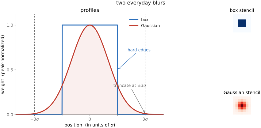
Run both on an actual photograph and the difference in feel is plain: the box smears fine texture into faintly blocky, slightly directional mush, while the Gaussian dissolves it smoothly and isotropically. Use a Gaussian when the blur should look natural (Figure 6.2.13).
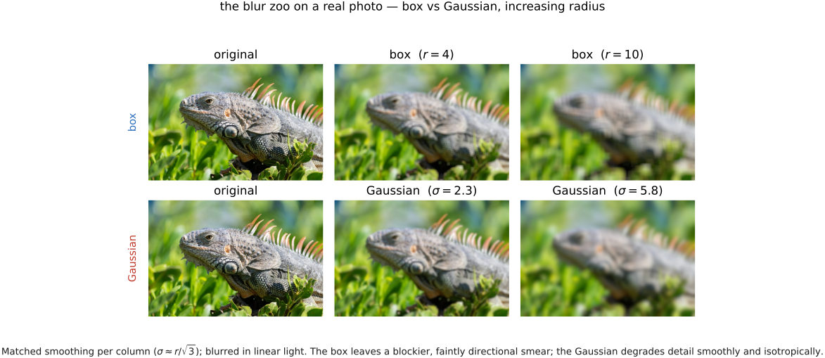
Better than reading about them, you can try the blurs directly (Figure 6.2.14): switch kernels, change the width, and watch what each does to real texture.
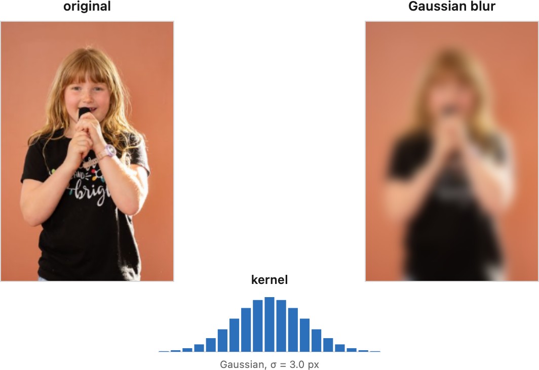
An ideal Gaussian has infinite support. At a distance $3\sigma$, its weight is $e^{-9/2}\approx0.011$ of the peak; a one-dimensional cut at $\pm3\sigma$ discards about 0.27% of the mass. Choose support for the required accuracy and renormalize the sampled, truncated weights. Square truncation preserves separability; circular truncation generally does not. Sampling and truncation make rotational symmetry approximate.
To simulate physical mixing, decode to linear light, filter, then encode for display. Aesthetic smoothing can deliberately use another space, but it should be named. Linear-light processing is essential when the blur is part of a calibrated forward model. For images with transparency, filter premultiplied color and alpha consistently to avoid color bleeding from transparent pixels.
The visible encoding error is easiest to see where black meets white. Averaging their encoded values gives a middle code value; decoding that value generally yields less light than averaging the original linear intensities. A blurred highlight can therefore acquire a dark transition when filtering is done in the display encoding. The arithmetic is still linear in the stored numbers, but it no longer represents linear mixing of light.
6.2.7 Separability⧉
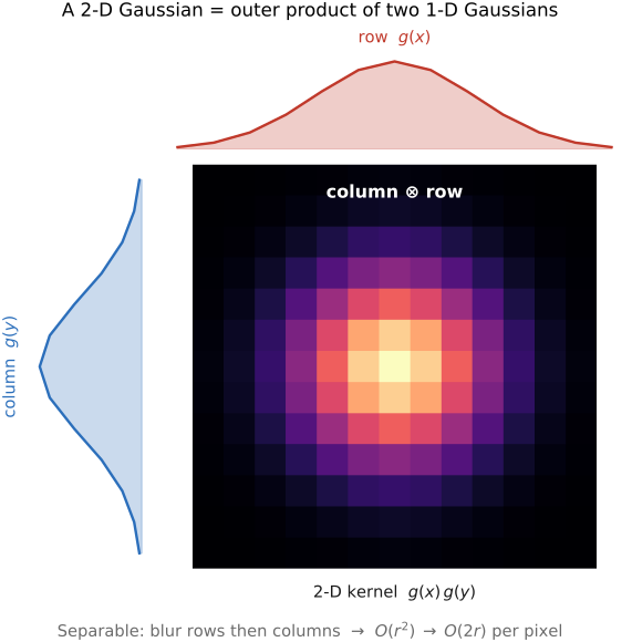
A $(2r+1) \times (2r+1)$ Gaussian appears to cost $(2r+1)^2$ multiplies per output pixel, quadratic in the radius, which is painful for a big blur. There is a shortcut. A 2-D filter is separable if it can be written as one 1-D filter applied along the rows followed by another along the columns, formally, the 2-D kernel is the outer product of two 1-D kernels. The Gaussian is separable, because $\exp(-(x^2 + y^2)/2\sigma^2) = \exp(-x^2/2\sigma^2) \cdot \exp(-y^2/2\sigma^2)$: a 2-D Gaussian is a horizontal 1-D Gaussian times a vertical one.
This is a genuine speedup. Instead of one $(2r+1)^2$ pass you do two $(2r+1)$ passes: blur every row with a 1-D Gaussian, then blur every column. The cost per pixel drops from $O(r^2)$ to $O(2r)$, linear in the radius. For a $\sigma = 10$ Gaussian (radius 30, a 61×61 kernel) that is the difference between ~3700 multiplies per pixel and ~120, about 30 times fewer multiplications, before accounting for memory traffic and implementation overhead. Separability is the first of several "do it in 1-D twice" tricks that recur through the book.
In code it is just two 1-D convolution passes with a scratch buffer between them:
# separable 2-D convolution: g = g_row ⊗ g_col, each 1-D and centered on zero
# pass 1: convolve every row with g_row
for each pixel (x, y):
    tmp[x, y] = 0
    for each offset x':
        tmp[x, y] += in[x + x', y] · g_row[-x']
# pass 2: convolve every column of the result with g_col
for each pixel (x, y):
    out[x, y] = 0
    for each offset y':
        out[x, y] += tmp[x, y + y'] · g_col[-y']
The box blur is separable in exactly the same way: an $n \times n$ average is an $n$-wide average along the rows followed by an $n$-wide average along the columns, so it too drops from $O(r^2)$ to $O(2r)$. Separability is a special property, though, not a universal one. A kernel factors like this only when it is rank one, its grid of weights being the outer product of a single row and a single column; a general kernel is not. The disk-shaped blur of a defocused lens is not separable, and neither is a diagonal motion streak, so those need the full 2-D sum or a different fast route (often the Fourier transform of the next chapter).
6.2.8 Linear sharpening⧉
Blur mixes a pixel with its neighbors; sharpening does the opposite, making each pixel more different from its neighbors. Where the image is flat the neighbors agree and there is nothing to do; where a pixel stands out, at an edge or a fine texture, sharpening exaggerates the difference so the feature reads crisper.
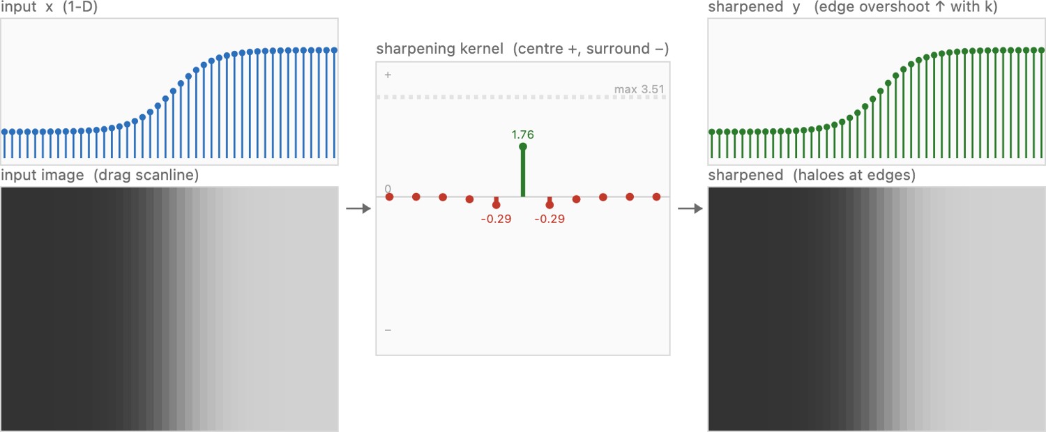
There is an equivalent way to say it that ties straight back to blur. A blurred copy of an image is its smooth, low-detail part, so whatever the blur removed is exactly the fine detail: $\text{detail} = \text{in} - g * \text{in}$. Sharpening is amplifying that detail, putting it back with a gain $k$:
This is the unsharp mask, and because every piece is linear it collapses to a single convolution,
a kernel with a tall positive spike at the center (the identity $\delta$) minus a scaled blur around it: positive in the middle, negative in the surround. For a unit-sum blur, this kernel also sums to one and preserves a constant.
They form a small family, differing only in the blur $g$ (equivalently, the band of detail) they amplify:
- Unsharp mask. Take $g$ a Gaussian; $\text{in} - g*\text{in}$ is a high-pass, everything finer than the Gaussian, and its radius ($\sigma$) and amount ($k$) are the two sliders every photo editor exposes.
- Laplacian. At a one-pixel radius the classic sharpening kernel is a $+5$ center with four $-1$ neighbors (the identity minus the discrete Laplacian): the same idea at the smallest scale.
- Difference of Gaussians (DoG). Rather than one blur, subtract a wider Gaussian from a narrower one, $\text{DoG} = G_{\sigma_1} - G_{\sigma_2}$ with $\sigma_1 < \sigma_2$. This is a band-pass: it isolates one band of detail (features near a chosen scale) instead of all detail at once, so a DoG can boost medium-scale texture without amplifying the finest pixel noise. For nearby scales, a suitably scaled DoG approximates a Laplacian-of-Gaussian up to sign. It also supplies a simple model of center-surround responses and a filter for blob detection.
Sharpening with a DoG is then just
Because all of these are linear convolutions they inherit this chapter's machinery, separability included (each Gaussian factors into a row pass and a column pass). Two failure modes limit linear sharpening: it amplifies noise along with detail (noise lives in the same high band), and it overshoots strong edges into bright and dark halos. Curing those needs the nonlinear, edge-aware sharpening of Chapter 8.8, Sharpening.
6.2.9 Gradient and oriented filters⧉
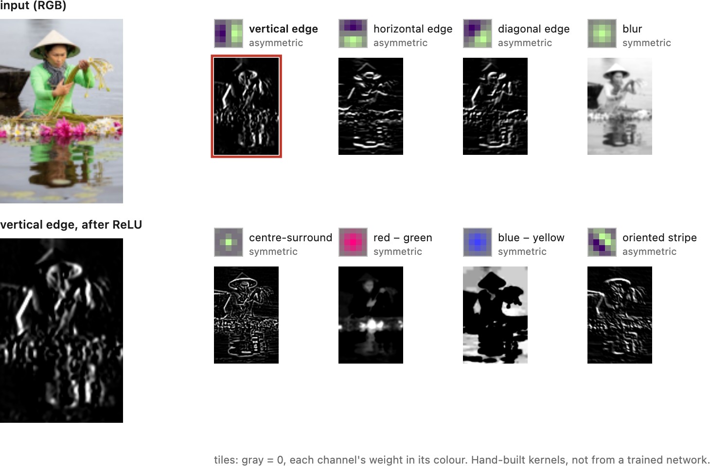
Not every useful kernel blurs. The most important non-blurring kernel measures change (how fast the image brightens or darkens as you step across it) and that turns out to be the foundation of edge detection.
With pixel spacing $h$, a forward difference is $I_x[i]=(I[i+1]-I[i])/h$. The weights $[-1,+1]/h$ act as a correlation stencil at offsets $0,1$. Under this chapter’s convolution convention, the same operation has $g[-1]=1/h$ and $g[0]=-1/h$. State the offsets as well as the weights: a two-tap stencil has no central sample. A ramp increasing to the right must produce a positive derivative.
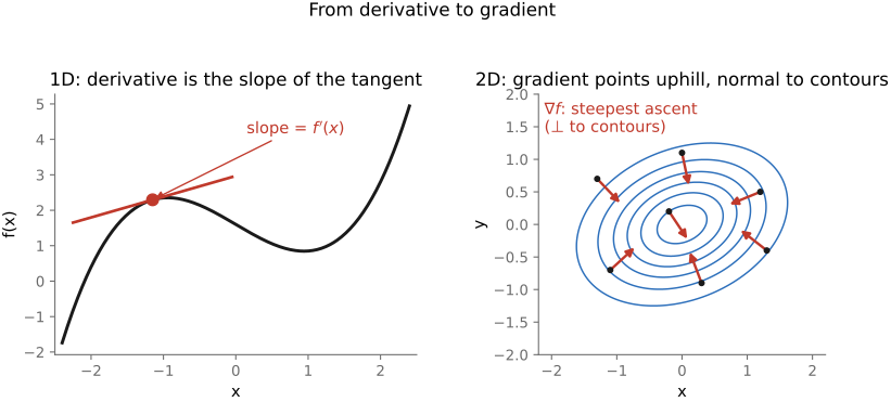
A grayscale image is a two-dimensional function (a brightness landscape with hills and valleys) so its derivative is not a single number but a gradient: a vector that, like the slope of a hill, points in the direction of steepest brightening and is perpendicular to the contours of constant brightness (Figure 6.2.17, right). Its two components are exactly the horizontal and vertical partials, $I_x$ and $I_y$, which is why we estimate each with its own finite-difference kernel.
Finite differences are convolutions with signed kernels under a declared indexing convention. In the continuous setting, $\partial_x(g*I)=(\partial_x g)*I$: convolving with a derivative-of-Gaussian differentiates a smoothed image. Gradient components are linear; gradient magnitude, thresholding, and a complete edge detector generally are not.
Differencing increases the contribution of rapidly varying noise. Sobel combines a difference along one axis with smoothing along the other. The following displayed matrix is a correlation stencil, using image coordinates with $x$ rightward and $y$ downward:
Divide its response by $8h$ to estimate a derivative in intensity per unit distance on a linear ramp. For convolution, flip the displayed stencil, which negates it. Its transpose gives the vertical stencil under the same convention.
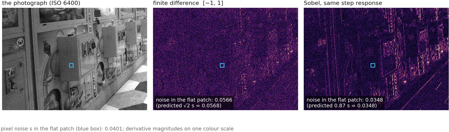
The smoothing is what Sobel buys. Scaled by 1/4, it gives a step edge the same height of response as the plain difference $[-1,\,1]$, but it averages three rows, weighted 1, 2, 1, before differencing. On independent pixel noise of standard deviation $s$, the plain difference has noise $\sqrt2\,s$ and the scaled Sobel $\sqrt{12}/4\,s\approx0.87\,s$, about 1.6 times less. The price is resolution: Sobel's response to an edge is two pixels wide (Figure 6.2.18).
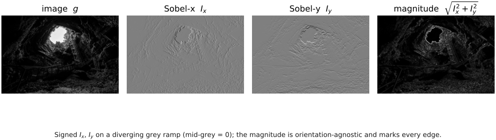
Stacking the two partials into a vector gives the image gradient $\nabla I = (I_x, I_y)$, the brightness-landscape gradient of Figure 6.2.17 applied to a real image. Two numbers fall out of it, both central to vision:
The magnitude is large at strong intensity changes, which can be object boundaries, texture, or noise. The gradient angle points across an edge; its tangent is perpendicular, $\theta+\pi/2$ modulo $\pi$. Thresholding magnitude gives a simple detector. Canny adds smoothing, non-maximum suppression, and hysteresis.
Blur, gradients, and sharpening all share the same comfortable assumption: one kernel, applied the same way everywhere. Before we lean on it, ask how well that assumption actually holds for the blur a real camera produces, because that is where the clean theory meets messy optics. (The linear sharpening above is only the start; its nonlinear, edge-aware forms are the Chapter 8.8, Sharpening chapter, and undoing a blur exactly, deconvolution, comes later still.)
6.2.10 Is imaging blur usually a shift-invariant convolution?⧉
This whole chapter has modeled blur as a convolution, one kernel, applied identically everywhere. How often is that actually true of real camera blur? Usually it is not, and knowing where the model breaks tells you when the clean linear-shift-invariant (LSI) tools apply and when they do not.
Camera rotation produces a sequence of homographies for a static scene and fixed intrinsics. Pan and tilt resemble translation over a narrow field, but their displacements vary across a wide image; roll traces arcs about the principal point. Camera translation introduces depth dependence and parallax. See Whyte et al. 2011/2014 and Chapter 16.4, Blind deblurring.
Defocus depends on the difference between a point’s inverse depth and the focused plane’s inverse depth, as well as the aperture and lens geometry. It is zero at the focused plane, not proportional to inverse depth alone. Visibility at foreground/background boundaries requires a fuller model than blurring each region independently.
Lens aberrations can vary with field position, wavelength, aperture, and focus. Coma and field curvature are important off-axis effects; spherical aberration is present on axis too. Longitudinal chromatic aberration shifts focus with wavelength. Lateral chromatic aberration shifts image position or scale with wavelength and can often be reduced by calibrated per-channel warps, though each broad color channel still integrates wavelength-dependent effects. See Chapter 22.1, Aberrations and optical challenges and Chapter 22.2, Aberrations correction.
Motion blur. Object motion blur follows each moving object's own trajectory (combined with the camera motion above), so different objects blur in different directions and amounts, again hard to model in 2-D at the boundary between a moving object and its background.
Diffraction is the well-behaved exception: the diffraction PSF (the Airy disk) is essentially shift-invariant across the frame, though some forms of vignetting (the aperture clipped by the lens barrel toward the corners, so not every pixel sees the whole aperture) modulate it off-axis.
Fixed software prefilters are convenient convolution models. Downsampling after a prefilter nevertheless discards information, and reconstruction filters do not generally undo that loss. A spatially varying resampling footprint is not one convolution over the original grid.
The pattern is clear: a real PSF can depend on (1) $1/\text{depth}$, (2) local motion, and (3) field (image) position, none of which a single shift-invariant kernel captures.
A convolution is an approximation when blur changes with depth, motion, field position, or wavelength. A small patch may support one kernel, but occlusion boundaries need particular care. Fixing geometry can preserve linearity in intensity even when shift-invariance is lost.
The difference between axial and lateral chromatic aberration changes the available correction. If wavelengths focus at different distances, a plane sharp in one channel may be blurred in another; aligning edges geometrically cannot restore the attenuated texture. If the principal difference is magnification, a per-channel warp can align much of the colored fringe. A broad channel still combines a range of wavelength-dependent magnifications, so even a successful alignment need not remove every within-channel smear. This is why the two effects should not be treated as one color-fringe problem.
6.2.11 Fixed and data-dependent weights⧉
A bilateral filter changes its weights with image values, so it is nonlinear. It can still be translation-equivariant on an infinite grid: translating the image translates the weights and result. Conversely, a fixed spatial mask is linear but not shift-invariant. These are separate properties, as Chapter 6.7, When linearity breaks down explains.
Chapter 6.3, Fourier analyzes fixed convolution kernels by frequency. Chapter 10.1, Bilateral filtering develops image-dependent weights for preserving boundaries while smoothing. Neither model is a universal description of neighborhood operations.
Recap: big lessons of this chapter
A convolution uses fixed weights that depend on displacement, not on image values or absolute position. On an infinite or periodic grid it is linear and commutes with shifts. The kernel can be small or span the image. Its support determines the work of direct filtering; finite boundaries determine where the shift-invariance model applies.
Convolution can be computed per output pixel or per kernel tap. In the first order we accumulate a neighborhood; in the second we accumulate shifted copies of the image. The result is the same. Replacing shifts with known warps gives other linear operators, but they need not share convolution’s commutativity or Fourier diagonalization.
Finite differences are convolutions with signed kernels under a declared indexing convention. In the continuous setting, $\partial_x(g*I)=(\partial_x g)*I$: convolving with a derivative-of-Gaussian differentiates a smoothed image. Gradient components are linear; gradient magnitude, thresholding, and a complete edge detector generally are not.
A convolution is an approximation when blur changes with depth, motion, field position, or wavelength. A small patch may support one kernel, but occlusion boundaries need particular care. Fixing geometry can preserve linearity in intensity even when shift-invariance is lost.