4.6 Sensing color: multiplexing strategies⧉
A bare photosite usually reports one integrated charge measurement, with a wavelength-dependent quantum efficiency, so to capture color we must somehow take three (or more) measurements where a given photosite provides only one. Every color camera multiplexes those measurements across some axis, and there are several ways to do it, each spending a different axis (Figure 4.6.1).
Strip away the color filter and a sensor is monochrome at the pixel: each photosite reports a single number, a signal proportional to detected photoelectrons within its operating range, not a color. The three (or more) values that color needs must therefore be multiplexed along some other axis: over space (a color-filter array such as Bayer, paying with resolution and a demosaicking step), over time (sequential color filters, paying with motion robustness: the old color-wheel and many scientific cameras), across multiple sensors (a beam-splitter prism feeding three chips, the 3-CCD video camera, paying with bulk and cost), or over depth (wavelength-dependent absorption in stacked photodiodes, the Foveon, paying with noise). The choice determines which measurements are simultaneous and co-located. The same constraint shapes the eye, whose three cone types sample color over space at the retina (L3.1, L3.6).
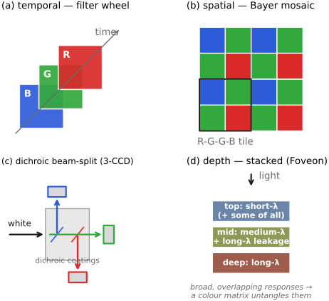
Three-channel color requires three distinct spectral measurements. Distributing them across space or time introduces assumptions about how the scene varies. Multiplex in time and you must assume the scene holds still between frames; multiplex in space and you must assume color varies smoothly enough to interpolate the samples you skipped; multiplex in depth and you inherit badly overlapping bands you then have to un-mix. A beam-splitter can send co-located, simultaneous images to several sensors, at the cost of alignment and optical complexity. A nanoscale router that sends wavelengths to neighboring photodiodes still uses spatial sampling.
4.6.1 Multiplexing in time⧉
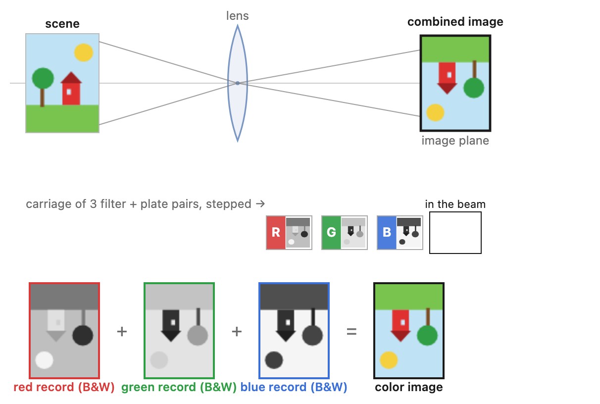
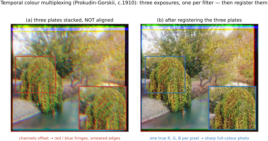
Shoot red, green, and blue frames sequentially through colored filters, or a rotating filter wheel. This is the principle behind Maxwell’s early color-photography demonstration (Maxwell 1861) and how Prokudin-Gorskii (Prokudin-Gorskii) captured the Russian Empire in three exposures. It is still how flatbed scanners, astronomy and fluorescence-microscopy filter wheels, telescope narrowband imaging, sequential-color machine-vision cameras, and many multispectral instruments work, because the same mechanism extends naturally from three filters to tens of narrow bands.
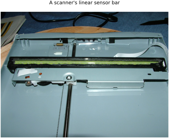
The implementations differ mainly in what does the sequencing. The oldest is a rotating filter wheel (or three separate plates) in front of a single sensor: three exposures through red, green, and blue filters, combined afterward. Maxwell’s 1861 tartan-ribbon demonstration and Prokudin-Gorskii’s later survey are early examples. Astrophotography still leans on it heavily: a cooled monochrome sensor (a mono sensor avoids the color filter array's light loss and keeps full resolution) sits behind a motorized filter wheel and stacks many long sub-exposures through each filter, red / green / blue for natural color or narrowband hydrogen, oxygen, and sulfur filters for nebulae, with tracking and registration to account for camera and celestial motion. Many flatbed scanners also scan spatially over time: a sensor bar is swept mechanically down the page, which is itself how a one-dimensional line sensor becomes a two-dimensional image (scanning spends time to buy the spatial axis the sensor lacks), and color can come from sequential illumination during a scan, separate passes, or spatially offset filtered sensor rows. Field-sequential color television and some endoscopes ran the same spinning-color-wheel trick in real time.
The trade-off is discrimination in time: the method assumes the scene and camera hold still across the exposures. For a static scene, each band uses the full sensor grid. The filters still reject light, and a fixed total capture time must be divided among bands. If the scene moves, its changing parts splits into colored fringes (Figure 4.6.6), and every temporal system must first register the plates to undo the small shifts between them (Figure 4.6.5), the simplest image-alignment problem in the book.
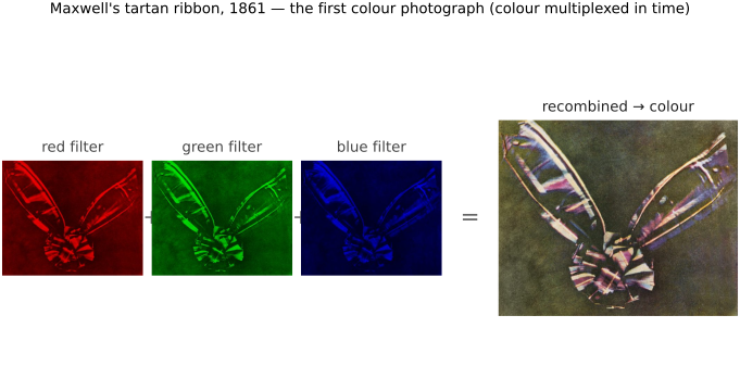
The three-color principle was demonstrated in 1861 by James Clerk Maxwell, the physicist who also unified electricity, magnetism, and light into the equations that bear his name. To demonstrate three-primary additive color reproduction, he had the photographer Thomas Sutton shoot a tartan ribbon three times through red, green, and blue liquid filters, then projected the three black-and-white positives back through the same three filters, superimposed, onto a screen. The overlap showed color in the celebrated 1861 demonstration, and a live demonstration of trichromacy, the same three-number logic the rest of this book rests on. It very nearly should not have worked: the wet-collodion plates of the day were almost blind to red and green, and the "red" record came mostly from ultraviolet that the ribbon's red dye happened to reflect. A lucky accident, but the principle was exactly right, with limitations imposed by the plates’ spectral sensitivity. (Maxwell 1861)
4.6.2 Multiplexing in space: the color filter array⧉
The dominant choice by far. Lay a color filter array (CFA) directly over the sensor so each photosite records one color and the missing two are filled in afterward by demosaicking (Figure 15.0.1, at the start of Part 15, Demosaicking and joint methods). The archetype is the Bayer mosaic, two green photosites for each red and blue, its doubled green mirroring the eye's green-weighted luminance (the eye is itself a spatial CFA, its interleaved cone mosaic). The family is large: Fujifilm’s X-Trans uses a repeating $6\times6$ tile that redistributes sampling artifacts; it does not eliminate aliasing; complementary CMY or CYGM (cyan-yellow-green-magenta) arrays pass more light through each filter than the primary RGB dyes; RGBW arrays add an unfiltered panchromatic "white" pixel for low-light sensitivity; and Huawei's RYYB swaps green for yellow to gather still more light. Phone sensors with many small pixels also group same-color photosites under one filter color. Quad-Bayer puts each color on a 2 × 2 block of photosites, and Nona-Bayer (Samsung's Nonacell) on a 3 × 3 block, so that a 108-megapixel sensor can combine each block of nine into one photosite and deliver a 12-megapixel image with less noise in low light, or read every photosite in good light. Chapter 15.5, Alternative color filter arrays covers how these layouts are demosaicked.
The reconstruction uses spatial and cross-channel regularity to estimate missing samples. Fine colored detail can violate those assumptions, producing false color and zipper artifacts. An optical low-pass filter can reduce aliasing at the cost of detail; not every camera uses one. A CFA also loses photons in its absorbing filters. Its practical advantage is simultaneous capture on one compact sensor.
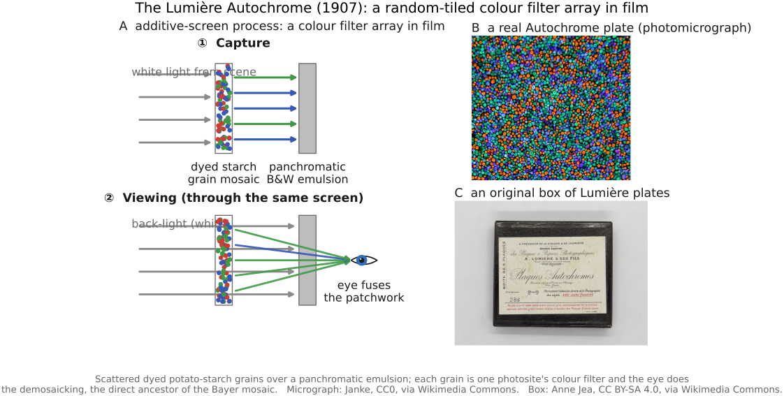
Color film reached the same spatial idea decades before silicon, by literally the same trick. The additive screen processes, the Lumière brothers' Autochrome (1907) and later Dufaycolor, Finlay, and Paget, coated the plate with a fine mosaic of transparent grains or patterned filters (Autochrome used orange-red, green, and violet-blue potato-starch grains; Dufaycolor printed a regular réseau grid) over a single panchromatic black-and-white emulsion. Each grain passed only its own color to the silver behind it, so the developed plate, viewed back through the same mosaic, rebuilt color from a spatial patchwork of filtered samples. This is a color filter array in film, the direct ancestor of the Bayer mosaic, decades before electronic CFAs, with each dyed grain filtering the emulsion behind it and vision integrating the fine mosaic at viewing distance. (The other film tradition, the stacked-dye integral tripack of Kodachrome and modern color film, multiplexes color in depth instead, and so belongs with the Foveon below.)
4.6.3 Multiplexing across separate sensors: the beam-splitter⧉
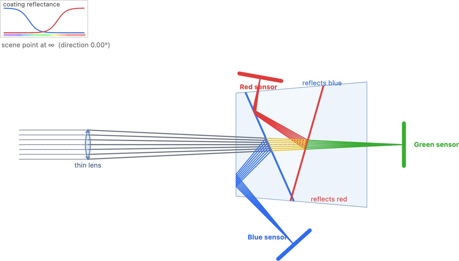
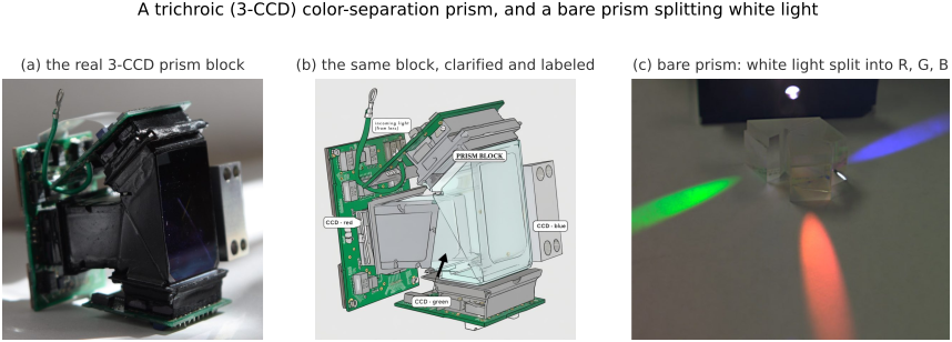
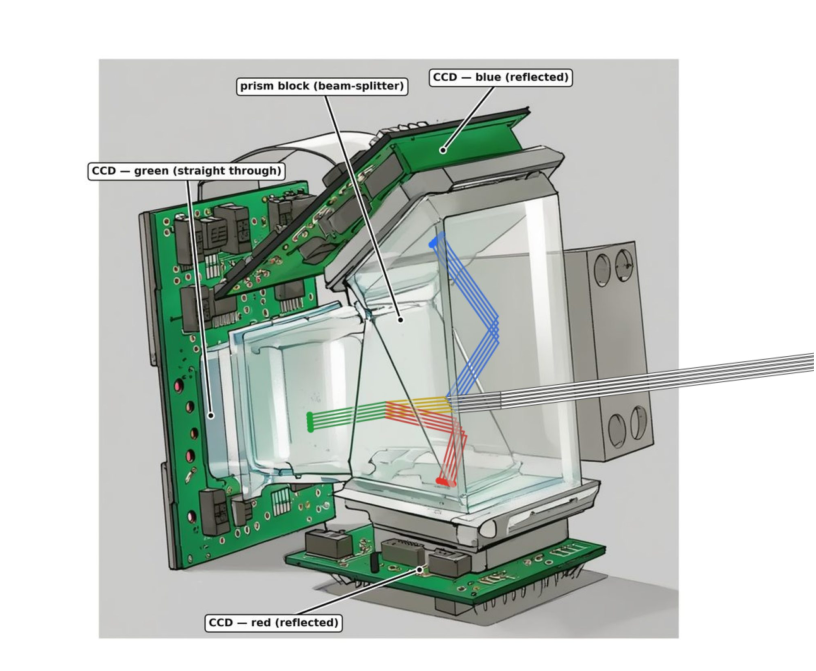
Send the whole image to more than one sensor and give each its own color. A dichroic prism block reflects each band onto its own chip (Figure 4.6.10): the 3-CCD / 3-chip design long standard in broadcast video cameras, three-chip cinema and telecine cameras, and scientific and machine-vision multi-sensor rigs. Because the dichroic coatings split the light rather than absorb it, the separation can retain more useful light than absorbing filters, and each channel has its own full sensor grid. (It is a dichroic beam-splitter, not a dispersing prism: it peels off three clean bands, it does not smear a spectrum.)
This strategy spends no scene axis, so it makes none of the constancy or smoothness assumptions of the other two: simultaneous sampling on three full grids without CFA demosaicking. Instead you pay hardware complexity: three sensors registered to sub-pixel accuracy behind a bulky, expensive prism. Bulk, optical tolerances, and cost limit its use. Adding bands increases the complexity.
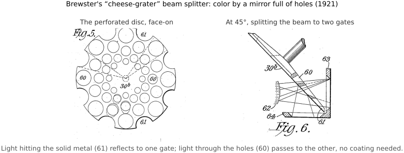
The hardware-splitting idea predates its dichroic form. Before interference coatings existed, P. D. Brewster’s historical beam splitter divided a movie camera's beam with a polished metal disc drilled full of holes (Figure 4.6.8): light passing through the holes went straight to one color film gate, while light striking the solid metal between them reflected off to a second. It is the cheese-grater ancestor of the 3-CCD prism, the same bargain of spending hardware rather than a scene axis so that each color gets its own sensor. It was cruder in two ways: the fixed metal-to-hole ratio sets a single reflect/transmit split rather than a wavelength-selective peel, and because the disc splits by geometry and not by color, each path still needs its own color filter. So it lacks the dichroic prism's wavelength-selective separation, but the core move is identical.
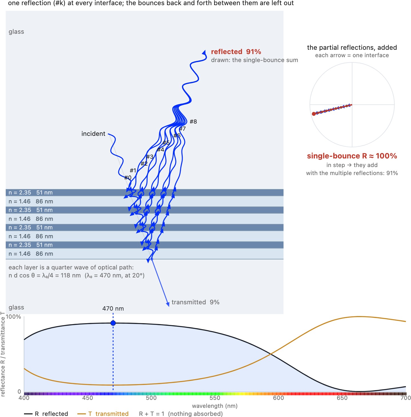
A dichroic coating separates bands through interference. The answer is the same interference that colors a soap bubble (Figure 2.1.33), run deliberately and many times over. The coating is a quarter-wave stack: alternating layers of a high- and a low-index transparent material, each with optical thickness $n_jd_j=\lambda_0/4$ at normal incidence in the simple quarter-wave design. Every interface reflects a little, and at $\lambda_0$ those weak reflections all come back in phase and add into a near-perfect mirror; outside the reflection band the coating transmits more light, with the detailed spectrum set by its complete layer design. In an ideal lossless coating, reflectance plus transmittance is one. Real stacks also have absorption, scattering, angular dependence, and polarization dependence (Figure 4.6.9).
4.6.4 Multiplexing per pixel by dispersion: color routers and nano-prisms⧉
A color router directs wavelength bands toward different photodiodes instead of rejecting unwanted bands with absorbing filters. Demonstrations range from dielectric splitters Nishiwaki et al. 2013 to inverse-designed structures Zou et al. 2022. The target is better photon utilization, but reported efficiency depends on wavelength, incidence angle, polarization, aperture, and the definition of useful detector area. One-third transmission is a teaching approximation for idealized equal-width RGB filters, not a universal CFA ceiling.
Routing to neighboring photodiodes still multiplexes color in space. The spatial response must be included in reconstruction; spreading light is not automatically a correctly designed anti-aliasing filter. Fabrication tolerances and off-axis response also matter. Commercial microlens or nanostructure enhancements that retain color filters should be distinguished from filter-free research routers.
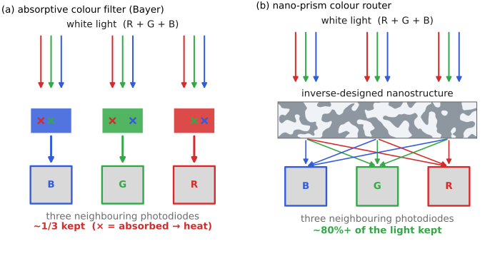
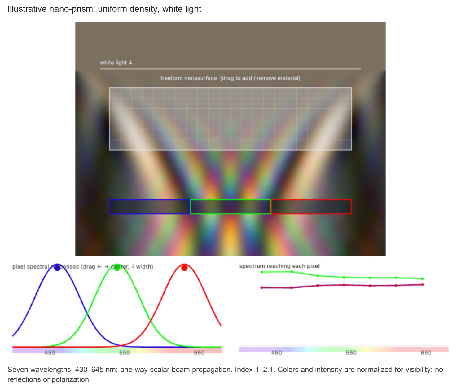
The comparison with a dichroic prism is useful, provided we keep track of the image coordinates. A prism can send complete registered images to separate sensors. A small router sends different wavelengths toward different sites within a local footprint. The latter can avoid absorbing some of the photons that a dye would reject, but neighboring detectors now receive contributions shaped by the router's wavelength-dependent spatial response. The reconstruction must know both which wavelengths and which scene locations contributed. Improving light collection and preserving spatial detail are therefore coupled design tasks, not two independent benefits of replacing a filter.
4.6.5 Multiplexing per pixel by tunable absorbers: quantum dots⧉
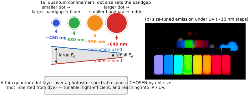
Colloidal quantum dots offer size- and material-dependent bandgaps and can form photosensitive layers above a readout circuit. They are useful research and device materials for spectral ranges and integration schemes that differ from silicon. Color-selective layers still need multiple independent measurements, whether distributed spatially or stacked.
A tunable bandgap does not imply an arbitrarily narrow absorption spectrum. Quantum dots can absorb broadly at energies above the band edge, even when their fluorescence is narrow. Nor does replacing a dye with another absorber automatically recover rejected photons. Evaluate absorption, charge extraction, dark current, stability, and cross-channel separation for the proposed architecture.
4.6.6 Multiplexing in depth: stacked photodiodes⧉
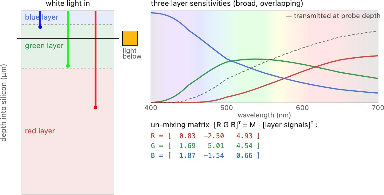
Stacked photodiodes use silicon’s wavelength-dependent absorption depth. Short wavelengths are absorbed near the surface; longer wavelengths penetrate farther. The layer signals overlap spectrally, so they require a calibrated color transform rather than being direct red, green, and blue measurements. Foveon designs use this principle; some variants sample deeper layers at lower spatial resolution and still require reconstruction. Noise after color correction depends on the measured layer sensitivities, collection efficiency, and covariance.
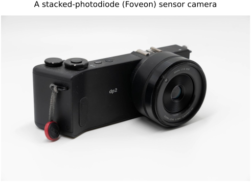
Few production cameras have ever used a Foveon sensor; the Sigma dp series is the best known (Figure 4.6.16), sold on exactly the trade above: unusually crisp, demosaicking-free luminance detail in exchange for noisier color, device-dependent sensitivity and readout limits.
For a simplified collection interval from depths $z_1$ to $z_2$, Beer–Lambert absorption gives the fraction $e^{-\alpha(\lambda)z_1}-e^{-\alpha(\lambda)z_2}$, where $\alpha$ is silicon’s absorption coefficient. This illustrates overlapping depth responses (Figure 4.6.17). Real charge collection also depends on device structure and carrier transport. A broad overlap can make some color distinctions noisy; quantify that through the calibrated transform rather than an invented “unmixing” matrix.
Depth multiplexing is not a silicon invention; color film got there first, chemically. The dominant color-film design, the integral tripack of Kodachrome, Ektachrome, and typical C-41 color negatives, stacks three color-sensitive layer groups, often containing several emulsions, on one base: a blue-sensitive layer on top, then a green-sensitive layer, then a red-sensitive layer, with a thin yellow filter layer just below the top one to stop stray blue (to which all silver halides respond) from leaking into the lower layers. White light enters the top and is caught band-by-band with depth, a similar stacked layout, though spectral sensitization in film differs from absorption-depth separation in silicon, and after development each layer forms its own complementary dye so the stack yields full color at every point with no spatial mosaic (Figure 4.6.18). It is the same trade the Foveon makes and the same one the Autochrome does not: color multiplexed in depth (stacked, full-resolution, no demosaicking) rather than across space (a mosaic that must be interpolated). Silicon's Foveon is the integral tripack rebuilt in a semiconductor, absorption depth standing in for the sensitized layers.
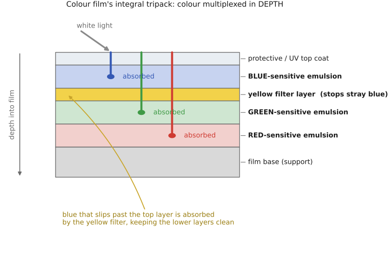
The depth layers are not three bins labeled blue, green, and red. Absorption is probabilistic: at a given wavelength, some photons are absorbed near the surface and others penetrate farther. A shallow collection region therefore receives longer-wavelength contributions as well as short-wavelength ones; deeper regions measure the surviving mixture. The equation above computes the difference between the fractions that reach the top and bottom of an idealized collection interval. This is why three layers need a calibration rather than merely being renamed RGB. When a desired color distinction changes the layer signals only slightly, recovering it can require a large difference of noisy measurements, connecting the sensor architecture to the matrix-noise calculation in Chapter 4.4, RGB color spaces.
4.6.7 Hybrid strategies⧉
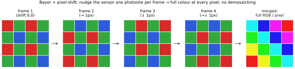
Real cameras often combine strategies, and the most useful hybrid is Bayer plus pixel-shift (Figure 4.6.19). A sensor-shift actuator moves through a specified sequence of one-photosite offsets, so that over four exposures every output location is sampled through a red, a blue, and both green filters in turn; merge the four and you get true R, G, B at every pixel with no demosaicking guesswork (full color resolution and additional samples for noise reduction) at the cost of needing a static scene on a tripod. (It is the spatial Bayer trick borrowing the temporal axis to fill its own holes.) Subpixel offsets can support super-resolution if the optics retain the detail and registration is accurate. Motion and occlusion require detection or fallback processing; more frames also mean more capture time. Video pipelines hybridise the other way, leaning on motion across frames; astrophotography filter wheels are temporal multiplexing with cooled sensors.
4.6.8 Beyond trichromatic capture: full spectrum and multispectral⧉
Multispectral instruments acquire more than three bands; hyperspectral systems sample many closely spaced bands. Filter wheels, scanned spectrometers, filter mosaics, and snapshot spectral encodings trade spectral detail against spatial sampling, time, and noise. A spectral cube is still a finite set of measurements with a calibrated spectral response, not an exact continuous spectrum.
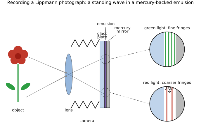
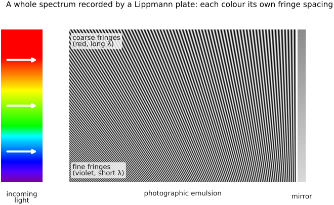
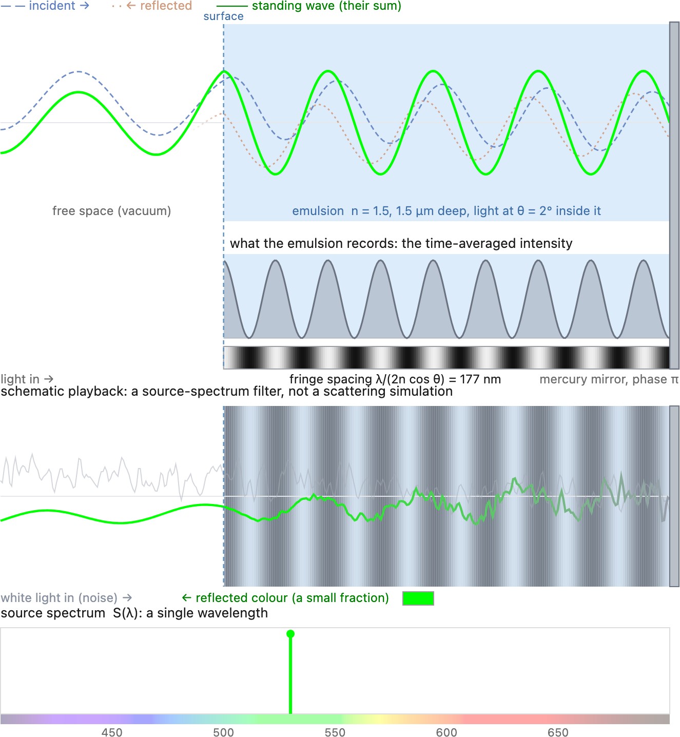
Lippmann photography records spectral information through interference along the depth of an emulsion Lippmann 1891 Lippmann color photography (Alternative Photography) Bjelkhagen, "Lippmann photography". Incident light and its reflection from a backing mirror form depth-dependent intensity fringes. For vacuum wavelength $\lambda$, refractive index $n$, and internal angle $\theta$, adjacent intensity maxima are separated by
After development, the layered structure selectively reflects wavelengths under suitable viewing illumination. Finite thickness limits spectral resolution; the mirror’s phase response, emulsion response, processing shrinkage, and viewing angle affect reproduction. It preserves more spectral information than an RGB photograph, but not a perfect, unlimited record of the original spectrum. Modern recovery methods model these distortions Baechler et al. 2021.
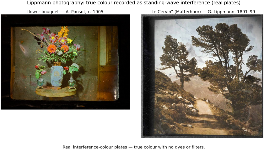
Gabriel Lippmann (1845–1921) received the 1908 Nobel Prize in Physics for interference color photography, the only Nobel awarded for a color-photography process. He was a physicist's physicist: his capillary electrometer was used to record the first human electrocardiogram, he predicted the converse piezoelectric effect that the Curies then confirmed, and he proposed integral photography, an ancestor of light-field imaging. Long exposures and restrictive viewing conditions limited the color process’s practical adoption, but its spectral recording remains an instructive alternative to trichromatic capture.
For a monochromatic exposure, the incident and reflected waves establish a repeated intensity pattern through the depth of the emulsion. Development records that pattern as a layered optical structure. When white light later illuminates it, reflections from successive layers reinforce one another near the recorded wavelength under the appropriate viewing geometry. A more complicated incident spectrum leaves a more complicated depth pattern. The layer spacing carries spectral information even though the emulsion is not divided into conventional red, green, and blue channels. Lippmann's method is therefore a useful counterexample to the assumption that a color photograph must store three numbers: it records another kind of optical measurement, whose reconstruction still has finite bandwidth and physical imperfections.
4.6.9 Spectral sensitivity: matching the eye, catching photons, and white balance⧉
With photon spectral exposure $q(\lambda)$ and effective channel detection probability $\eta_i(\lambda)$, the expected signal electrons are
The response includes filters, optics, and quantum efficiency under the stated convention. Sampled implementation needs wavelength-bin weights. Shot noise is determined by detected electrons, while read noise is added by the readout; the full model is in Chapter 2.8, Noise, signal-to-noise ratio and dynamic range. A broad response alone is not a color measurement: distinct response shapes supply the information that separates spectra.
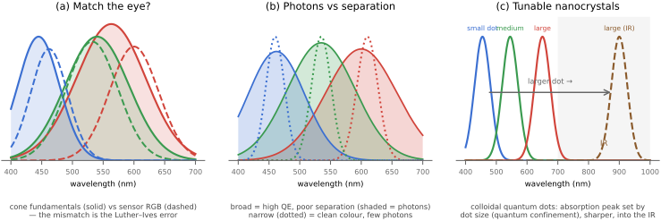
The exact shape of a color sensor's three spectral-sensitivity curves (the $r(\lambda)$ of the red, green, and blue channels, built earlier by the color-filter array on the photosites of Chapter 2.7, Sensors: photosites, CCD vs CMOS) is one of the camera's most constrained choices, because it is pulled in three directions at once that cannot all be satisfied.
- Fidelity to human vision. For a camera to record the color a human would see, its three curves should be a fixed linear combination of the eye's cone fundamentals (equivalently, of the CIE color-matching functions), the Luther–Ives condition. A sensor that met it could be mapped to human color by a single $3\times3$ matrix with no error. Practical camera sensitivities generally only approximate it, because silicon-plus-dye curves are simply the wrong shape, and the penalty is a metameric error no color matrix can remove: two spectra that look identical to the eye read as different RGB, and two that look different can read the same. The color-correction matrix in Chapter 8.10, Auto-exposure and auto white balance is a least-squares compromise: right on average, wrong on the hard cases (saturated reds, narrow-band LEDs, foliage).
- Quantum efficiency and noise. Broad transmission bands can increase total photon collection; this is distinct from quantum efficiency at a specified wavelength: the wider each filter, the more photons reach the well and the higher the SNR. Strong overlap can make color separation poorly conditioned, because separating similar channel responses can require large signed coefficients that amplify measurement noise (compare the distinct physiological opponent processing in Chapter 3.2, Perceptual color and trichromatic vision). Narrow, well-separated filters give clean color but throw photons away and read noisier. The green-doubled Bayer is one point on this curve: spend photons and resolution where the eye cares most (luminance), economize on chroma.
- White balance across illuminants. Because each channel integrates illuminant × reflectance × sensitivity, changing the light changes the raw RGB of a fixed object. Undoing that, white balance often approximates the change with per-channel gains. Matching cone sensitivities does not make this diagonal relighting model exact; a response set that matches human colorimetry well need not be the best basis for diagonal adaptation. Good spectral design makes white balance more reliable across illuminants (→ Chapter 8.10, Auto-exposure and auto white balance).
These three pull against each other: the curves that best match the eye are broad and overlapping (bad for separation), the curves that separate color cleanly are narrow (bad for QE and for matching the eye), and keeping white balance stable across odd illuminants wants yet another shape. Every color sensor is a negotiated settlement among them (Figure 4.6.24).
Recap: big lessons of this chapter
Strip away the color filter and a sensor is monochrome at the pixel: each photosite reports a single number, a signal proportional to detected photoelectrons within its operating range, not a color. The three (or more) values that color needs must therefore be multiplexed along some other axis: over space (a color-filter array such as Bayer, paying with resolution and a demosaicking step), over time (sequential color filters, paying with motion robustness: the old color-wheel and many scientific cameras), across multiple sensors (a beam-splitter prism feeding three chips, the 3-CCD video camera, paying with bulk and cost), or over depth (wavelength-dependent absorption in stacked photodiodes, the Foveon, paying with noise). The choice determines which measurements are simultaneous and co-located. The same constraint shapes the eye, whose three cone types sample color over space at the retina (L3.1, L3.6).