4.5 Advanced color: opponents, perceptually-uniform, and preferred⧉
Color picking, perceptual difference measurement, and preferred rendering need more than RGB coordinates. This chapter develops representations and models for those tasks, with the conditions under which their predictions are useful.
4.5.1 Opponent color spaces and separating luminance and chrominance⧉
Opponent representations separate an achromatic coordinate from two color-difference coordinates. This is useful for compression because chromatic spatial resolution is often lower than luminance resolution. Chroma subsampling still produces visible artifacts on colored text, graphics, and fine edges; the advantage is a tradeoff rather than a free reduction.
YCbCr applies a matrix to specified nonlinear RGB values, with offsets for storage. It is affine in the encoded coordinates and nonlinear with respect to light. YUV is related but has different definitions and scaling. Specify the matrix coefficients, full or limited range, bit depth, and chroma sampling and siting when reading either format.
A common full-range, Rec. 601-style YCbCr conversion for normalized encoded RGB is:
and the inverse recovers the primed channels,
The printed coefficients are rounded. The offsets center neutral chroma at 0.5 in this normalized convention; integer formats may specify a center such as code 128 and distinct scale factors. Do not substitute these floating conventions for a codec’s exact integer mapping.
YCbCr’s luma is a weighted sum of nonlinear channels. It supports coding and chroma subsampling but is not photometric luminance. Chroma errors can change decoded luminance as well as color. Decode into a defined linear space for a radiometric calculation.
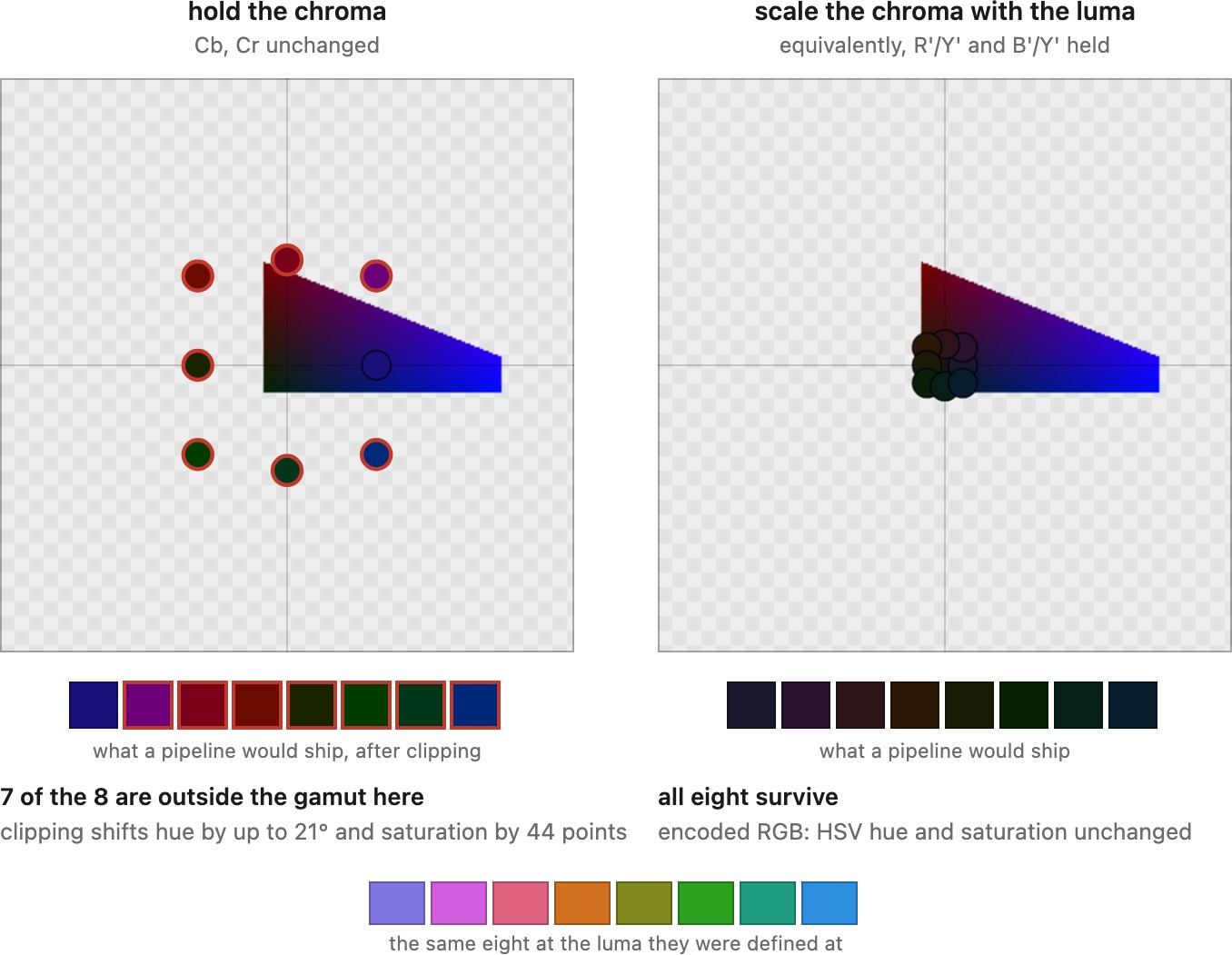
A large luma edit at fixed chroma differences can move values outside the RGB gamut. If the objective is to change linear luminance from $Y$ to $Y_t$ while retaining chromaticity, a direct operation is
Handle black separately and decide how to map values beyond the output range. This preserves XYZ chromaticity before gamut mapping, not necessarily perceived saturation under changed viewing conditions. A log-luminance representation is convenient for specifying $Y_t$, but is not required to implement the scaling.
DKL describes calibrated opponent directions relative to an adapting background Derrington, Krauskopf & Lennie 1984 (DKL cardinal directions). Its exact coefficients depend on cone fundamentals and normalization; the equal-weight teaching model in Chapter 3.2, Perceptual color and trichromatic vision is not a universal calibration. IPT targets useful hue behavior Ebner & Fairchild 1998 (IPT). ICtCp, specified in Rec. 2100 ITU-R BT.2100 (HDR-TV; ICtCp), applies a nonlinear transfer to a defined LMS-like intermediate before forming opponent coordinates. PQ and HLG variants have specified transforms. These improve aspects of HDR coding but do not guarantee unchanged appearance under arbitrary independent channel edits.
A color-difference magnitude depends on signal scale. In a linear opponent representation, scaling luminance and both centered chroma components together preserves the underlying chromaticity. Ratios describe that algebra, but a ratio such as chroma divided by luminance is not a universal perceptual saturation formula. State what the edit preserves.
A large brightness edit exposes the difference between keeping chroma differences fixed and keeping color ratios fixed. Suppose all three linear RGB values of a pixel are halved. Its chromaticity stays the same because their proportions stay the same. If instead only a luma coordinate is halved while additive chroma coordinates remain fixed, converting back can change those proportions and can drive a channel negative. That matters in HDR tone mapping, where the brightness change may be large. The representation should express what the edit intends to preserve; separating channels does not by itself make their meanings independent.
Holding luma fixed does not, in general, hold physical luminance fixed. Change a chroma value while keeping $Y'$ unchanged, convert back to encoded RGB, and decode the channels. The nonlinear decoding can change the weighted sum of linear RGB even though the weighted sum of encoded RGB stayed constant. Chroma subsampling can therefore affect luminance as well as color near an edge. The separation is useful for compression, but the labels on its channels do not make it a physically independent brightness-and-color representation. This is one motivation for studying alternative HDR component encodings.
4.5.2 Tensions: linearity, gamma, and opponents⧉
Three distinctions organize these spaces. First, a numerical coordinate can exist without being physically realizable or displayable. Second, a transform can be linear in encoded coordinates without being linear in light: YCbCr is the standard example. Stored sRGB is not a linear transform of XYZ; its linearized version is. Third, a convenient representation for storage or selection need not have useful perceptual distances.
A color-space choice should follow the calculation: physical mixing, compression, interactive selection, and difference measurement are different jobs. No single opponent split solves all four.
4.5.3 HSV, HSL, and cylindrical color spaces⧉
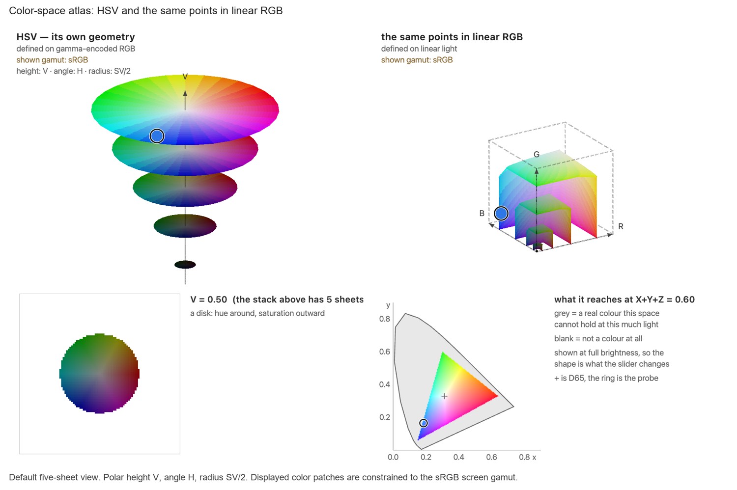
HSV and HSL provide convenient color-picker controls: hue, a saturation parameter, and either value or lightness. Their names borrow perceptual vocabulary, but their axes are arithmetic on RGB. A saturated yellow and a saturated blue can have equal value without equal luminance or lightness.
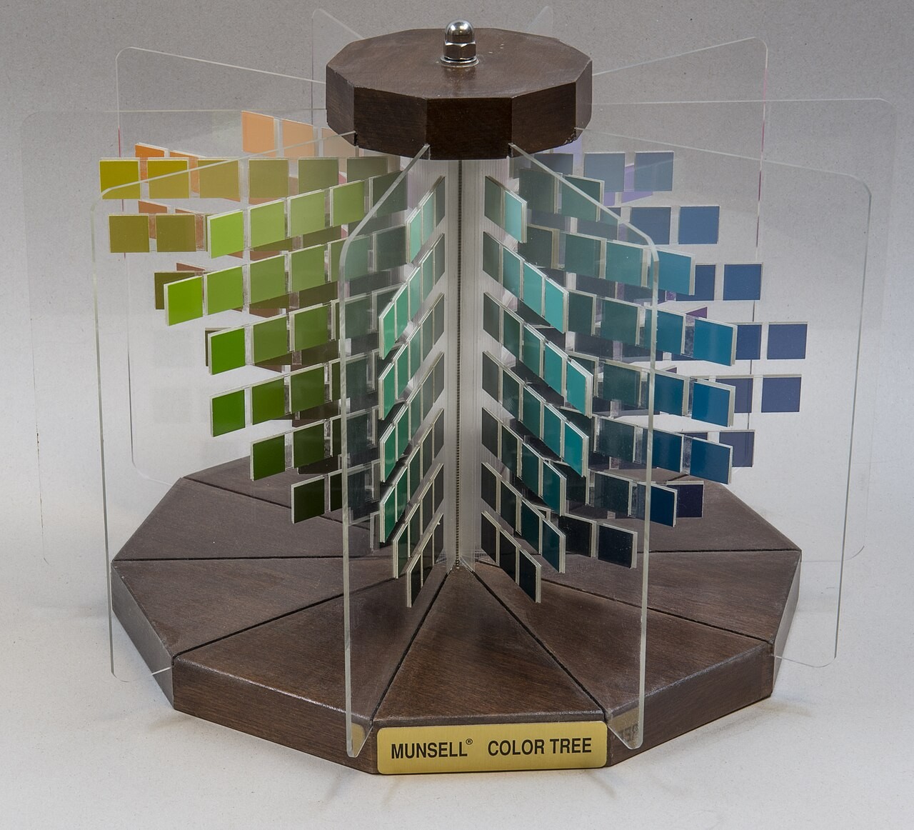
Munsell’s hue/value/chroma organization was instead developed through visual judgments. Its irregular color tree is a useful contrast to the regularized shapes used for software controls.
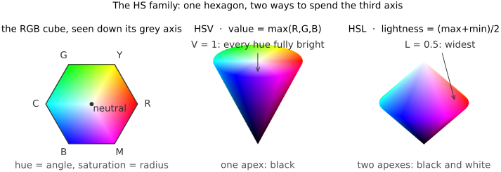
The usual HSV/HSL definitions operate on encoded RGB, inheriting its primaries, white reference, and transfer function. They can be computed on other triples, but that produces a different convention. Write the channels in $[0,1]$ and let $M=\max(R',G',B')$, $m=\min(R',G',B')$, and $C=M-m$ be the chroma, the spread between the brightest and darkest channel. The hue is identical in both spaces, the angle of whichever channel dominates, read most cleanly through the sextant coordinate $H' \in [0,6)$:
The two spaces differ only in the third axis and how they scale saturation to run from $0$ to $1$. HSV keeps the brightest channel as value $V=M$; HSL takes the midpoint as lightness $L=(M+m)/2$; each divides the chroma by a different denominator:
Both maps invert in closed form. Recover the chroma from the third axis, $C = V\,S_V$ for HSV and $C = (1-|2L-1|)\,S_L$ for HSL, form the intermediate $X = C\,\big(1 - |H' \bmod 2 - 1|\big)$, and place $C$ and $X$ into the RGB channels according to the hue sextant,
then add back the gray level the third axis fixes, $m = V - C$ for HSV or $m = L - C/2$ for HSL, giving $(R',G',B') = (R'+m,\,G'+m,\,B'+m)$. For achromatic colors, set a conventional stored hue or retain the previous UI hue; its physical value is undefined. Wrap hue before the inverse. Tie cases for the maximum agree away from the achromatic case.
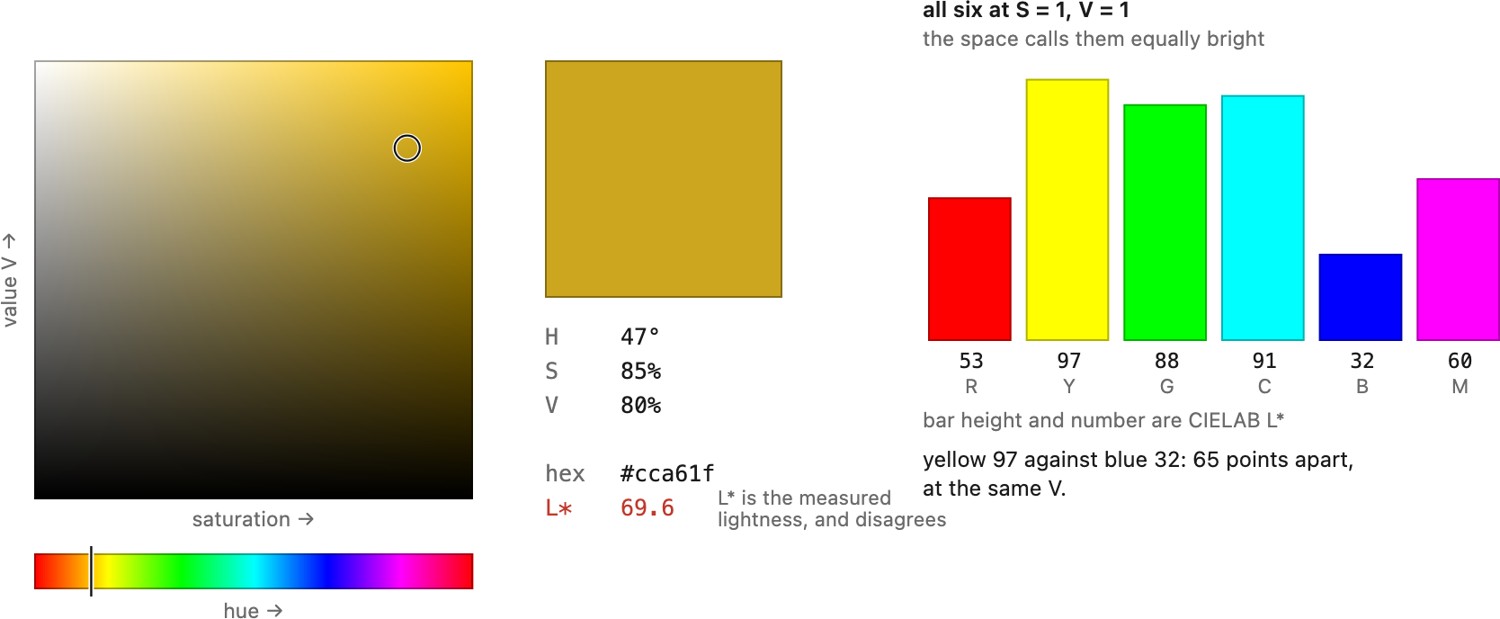
HSV can be useful for a task-specific threshold or UI selection. Do not interpret its Euclidean distances as perceived differences, or assume a hue threshold transfers unchanged across cameras and illumination. Hue wraps at the red boundary and becomes unstable at low saturation.
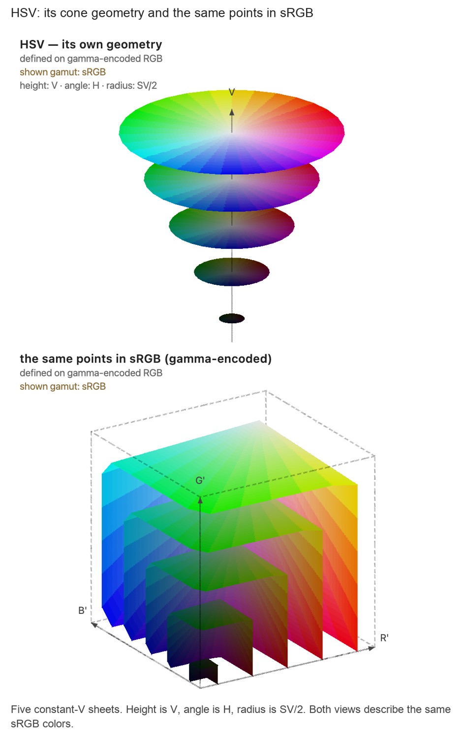
The apparent solid depends on what is plotted. In HSV, value is the maximum RGB component, so a constant-value sheet contains triples whose largest component has that fixed value. Saturation then measures the channel spread relative to it. Drawing hue as an angle and normalized saturation as a radius makes the controls look cylindrical; drawing chroma as the radius makes the available radius shrink toward black. The colors have not changed. They have been laid out according to different choices of coordinates. Munsell's irregular tree answers another question: how to arrange visually judged hue, value, and chroma steps. A tidy software control and a perceptually even arrangement need not have the same shape.
4.5.4 Perceptually uniform color spaces⧉
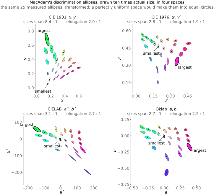
Matrices preserve straight lines but they do not make equal coordinate steps look equally different to the eye. A fixed numerical change in sRGB is a large perceived jump in some colors and an invisible nudge in others. MacAdam’s 1942 experiments provide an influential example of this nonuniformity (Figure 4.5.6). For tasks that need perceptual uniformity (color-difference tolerances, gradients, palette design), we need a deliberately non-linear space. The standard one is CIE L\a\b\ (CIELAB), which applies a cube-root compression of $XYZ$ about a reference white and recombines the result into a lightness axis L\ and two opponent chroma axes a\ (green–red) and b\ (blue–yellow):
The signature is $f_\mathrm{Lab} : \mathrm{XYZ}_{[\mathrm{D65}]} \to L^*a^*b^*$, and the input type is the trap: CIELAB is defined on linear XYZ (bare, unprimed symbols), so computing it straight from the primed $R'G'B'$ of a JPEG without first decoding to linear light and going through XYZ is a type error that quietly warps every $\Delta E$. Here $(X_n, Y_n, Z_n)$ is the reference white, for D65 and the CIE 1931 2° observer $(95.047,\,100,\,108.883)$, and the cube root carries a short linear segment below $\delta^3 \approx 0.0089$ to tame its infinite slope at black. In this space equal distances correspond, roughly, to equal perceived differences, so color difference is just a Euclidean distance, $\Delta E^*_{ab} = \lVert \Delta \mathbf{Lab} \rVert = \sqrt{\Delta L^{*2} + \Delta a^{*2} + \Delta b^{*2}}$ (with the refined ΔE2000 formula correcting the residual non-uniformities). Thresholds depend on the metric, stimulus, and viewing conditions; neither one nor 2.3 is a universal acceptance threshold. Use the same white normalization for the stimulus and $(X_n,Y_n,Z_n)$. The polar form gives the more intuitive chroma $C^*_{ab} = \sqrt{a^{*2} + b^{*2}}$ (distance from the neutral axis) and hue angle $h_{ab} = \operatorname{atan2}(b^*, a^*)$.
Its close cousin CIE L\u\v\* (CIELUV) keeps the same $L^*$ but scales chromaticity through the CIE 1976 uniform chromaticity coordinates $u', v'$:
with $(u'_n, v'_n)$ the white point's coordinates and $L^* = 116\,(Y/Y_n)^{1/3} - 16$ (again with the linear segment near black, $L^* = (29/3)^3\,Y/Y_n$ when $Y/Y_n \le \delta^3$). At black, set $L^*=u^*=v^*=0$ directly rather than evaluating the undefined chromaticity fractions. CIELUV is favored in lighting and display work because an additive mixture of two lights lies on a straight line in the $u',v'$ plane, but this does not make the full nonlinear Luv* transform additive (Berns, Principles of Color Technology).
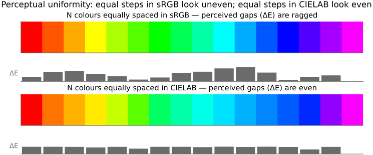
$XYZ$, $xy$, RGB, and HSV are built to measure and store color. Judging how different two colors look takes a space deliberately warped for that job, such as CIELAB (CIE 1976 (CIELAB)) with its $\Delta E$. Mixing the two up is why gamut areas on the $xy$ diagram mislead, why a gradient that is even in RGB banks unevenly to the eye, and why an error computed in the wrong space rewards the wrong thing. Ask of any color number: is this for measuring, or for judging?
The deeper reason a uniform space must be non-linear is the same reason gamma encoding exists: contrast sensitivity varies with stimulus level and chromaticity, so any space that turns perceived difference into geometric distance has to warp $XYZ$ accordingly (Figure 4.5.8). CIELAB is not the last word (it has known non-uniformities, especially in saturated blues), and a line of follow-ups refine it while keeping the same intent. The color-appearance-model variant CAM02-UCS (built on CIECAM02) and Björn Ottosson's Oklab (Ottosson 2020 (Oklab)) improve the perceptual uniformity and the blues; Chong, Gortler & Zickler's perception-based space (Chong et al. 2008) takes a different and, for our purposes, telling angle: it builds a color space from a small set of perceptual axioms and lands on a logarithmic construction that is designed so that, under a diagonal relighting approximation, a change of illuminant (which, recall, multiplies the spectrum, L2.6) becomes a simple translation in the space, so the differences image processing cares about are unchanged. That log structure is the same additive-vs-multiplicative theme that runs through tone mapping and exposure, here giving invariance to lighting; we use the Chong log space again in gradient-domain compositing.
DIN99 applies a rotation and logarithmic compressions to Lab to improve difference behavior under its fitted conditions. It is another named metric, not a drop-in identity with CIEDE2000. Use its complete specified variant instead of mixing constants across DIN99, DIN99b, and related definitions.
Oklab is worth writing out, because it is both better-behaved than CIELAB in the blues and cheap: two matrices around a cube root, defined on linear sRGB. With the signature $\mathrm{RGB}_{709} \to Lab_\mathrm{OK}$,
The displayed matrices are rounded; use the full published coefficients and real cube roots (including for signed inputs) in code. Oklab starts from linear light, so feeding it the primed $R'G'B'$ off a JPEG, a frequent shortcut, computes a different space than the one whose uniformity you wanted.
Concretely, Chong et al. prove that their axioms force the space into one shape, a linear map of the logarithms of a linearly recombined stimulus. With $\bar{x}$ in $XYZ$ and both matrices invertible and $3\times3$,
The two matrices have separate jobs. $B$ takes $XYZ$ to the basis in which relighting is best approximated by a per-channel multiplication, which is spectral sharpening again (Chapter 4.2, White balance and white point) and is fitted to spectral data. $A$ is then free, and they fit it to the RIT-DuPont and Witt perceptual-distance sets so that Euclidean distance approximates perceived difference.
The invariance falls out of the logarithm. Relighting is $\bar{x} \mapsto B^{-1} D B \bar{x}$ for a diagonal $D$, so in these coordinates it is $F(\bar{x}) + A\ln(\operatorname{diag} D)$: the same displacement for every color in the image. A change of light is a rigid translation of the whole space, which leaves every color difference untouched, and differences are what gradient-domain methods, segmentation and edge detection actually consume. The logarithm requires positive transformed components. This invariance holds for the assumed diagonal relighting model, not arbitrary spectral changes. Projecting out a single common-exposure direction would leave two dimensions; quotienting out all three independent gain directions would not.
For the original DIN99 transform with unit parametric factors, the lightness compression is
Rotate and scale the Lab opponent plane using $e=a^*\cos16^\circ+b^*\sin16^\circ$ and $f=0.7(-a^*\sin16^\circ+b^*\cos16^\circ)$. With $G=\sqrt{e^2+f^2}$, the chroma compression is $C_{99}=\ln(1+0.045G)/0.045$. For $G>0$, set $(a_{99},b_{99})=(C_{99}/G)(e,f)$; at $G=0$, set both to zero. Euclidean distance in the resulting coordinates defines the corresponding difference measure. The Color implementation gives these constants and the distinct refined variants.
The two logarithms have the same computational role, compressing a range, but their design objective is perceptual difference. The logarithm in Chong's construction instead makes an assumed illumination change act as a translation. Similar-looking formulas can serve different invariances; choosing one because it contains a logarithm misses the reason it was built.
4.5.5 Recap: a zoo of color spaces optional⧉
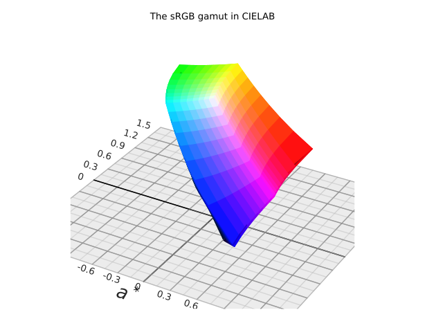
Plotting the same stimuli in several spaces reveals what each transform changes. Straight RGB lines can become curved in perceptual coordinates, and equal code steps need not have equal perceptual size. Keep the stimulus set fixed during the comparison. The whole realizable color cone, a bounded display gamut, and a bounded coordinate box are three different sets.
Y'CbCr), dynamic range at a chosen bit depth (8.0 stops for linear RGB, 11.7 for sRGB, 18.8 for ICtCp), how much luminance still hides inside one lightness, and how evenly the MacAdam ellipses come out.A display gamut and a coordinate system should remain separate in the picture. In linear XYZ, three fixed additive primaries with bounded independent intensities span a parallelepiped. In those primaries' own linear RGB coordinates, the same set is a cube. A nonlinear perceptual transform bends its faces without changing which stimuli the display can emit. The larger cone of physically realizable emitted colors is another set again: scaling a realizable spectrum by a positive factor keeps it realizable, whereas the display eventually reaches its intensity limits. Changing the plotted space changes the appearance of those sets, not the hardware limits.
4.5.6 Color appearance models⧉
A color appearance model predicts attributes such as lightness, brightness, chroma, colorfulness, saturation, and hue from tristimulus values and viewing conditions. CIECAM02 and CAM16 include adapting white, luminance, background, and surround parameters CIECAM02 Li et al., CAM16 and CAT16 (2017). Their uniform-space derivatives support color-difference calculations under specified conditions. iCAM and iCAM06 extend appearance modeling toward spatial images and HDR rendering. Among the effects these models encode are the Hunt effect (colorfulness rises with luminance), the Stevens effect (perceived contrast rises with luminance) and the Bezold–Brücke shift (hue changes with intensity), so one set of $XYZ$ values seen under a dim tungsten lamp and under bright daylight is predicted to look different, as it does.
These models are useful when viewing conditions are part of the task, including cross-media reproduction and some output-rendering systems. Their predictions depend on those inputs. A per-patch model does not by itself capture spatial adaptation or every image-context effect, and an unknown viewing environment remains unknown after calling the model. For simpler palette and difference tasks, a specified Lab or Oklab workflow may be sufficient. Fairchild Fairchild, Color Appearance Models, Hunt Hunt, The Reproduction of Color, and Reinhard et al. Reinhard et al., Color Imaging develop the distinctions.
4.5.7 Preferred colors: skin, sky, and other memory colors⧉
Viewers bring expectations to familiar objects, especially faces. A camera can produce a colorimetrically plausible image yet render a face in a way its subject dislikes. Skin rendering therefore requires both accurate measurement and a deliberate rendering objective.
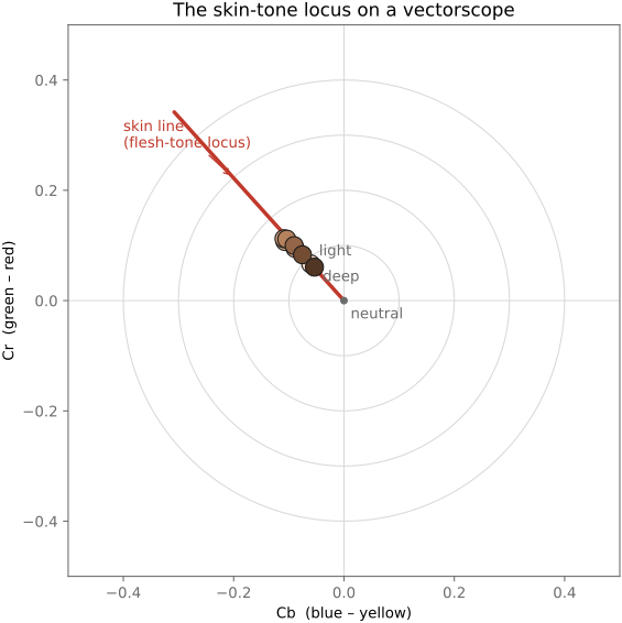
The vectorscope’s conventional skin-tone line is a useful reference under some lighting and rendering conditions. It is not a universal target. Complexions, blood perfusion, body site, illumination, makeup, exposure, and camera processing all affect the measured hue. Pulling every face toward one line can remove real variation.
CIELAB skin measurements must specify their illuminant and observer. The individual typology angle Chardon et al. 1991 (ITA°) is a descriptor based on $L^*$ and $b^*$, conventionally expressed as $\mathrm{ITA}=\arctan((L^*-50)/b^*)$ in degrees in its intended domain. It discards $a^*$ and is not a complete color description. Do not infer a person’s complexion category from an uncalibrated JPEG or treat fixed hue limits as an inclusive skin detector.
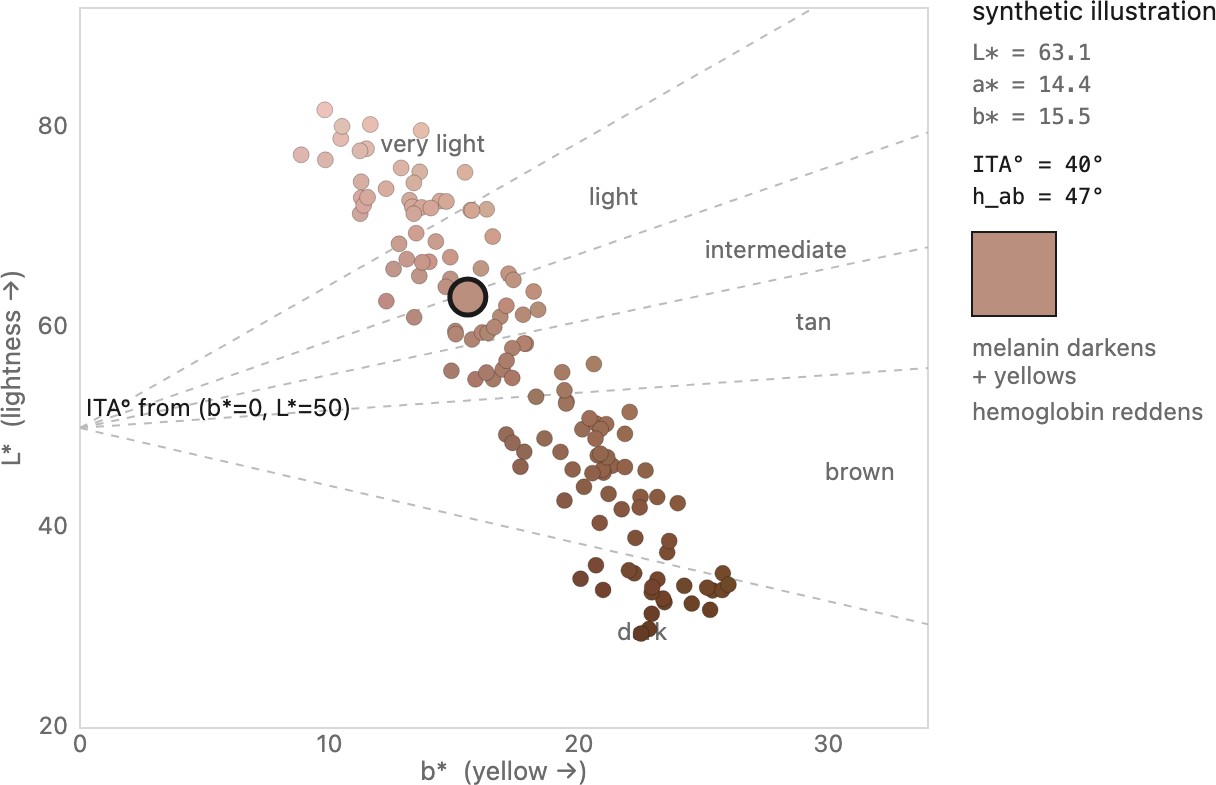
Melanin and hemoglobin strongly influence skin reflectance, but skin is not exactly a two-parameter color surface. Hemoglobin oxygenation, layer thickness, scattering, and illumination also matter. Tsumura et al. Tsumura et al. 2003 estimate pigment-related image components using a model and statistical assumptions; arbitrary RGB attenuation vectors are not that calibrated method.
A physical forward calculation keeps the spectral integration explicit:
reflectance = skin_model(wavelengths, pigment_parameters, scattering_parameters)
stimulus = illuminant_spectrum * reflectance
XYZ = integrate(stimulus * XYZ_matching_functions, wavelength)
RGB = render_for_display(XYZ, viewing_conditions)
A log-RGB approximation can simplify separation under suitable conditions, but the logarithm of a spectral integral is not the integral of a logarithm. Label any reduced model and validate it against measured spectra. For spatially resolved rendering, subsurface scattering also matters: a BSSRDF relates entering light at one surface point to exiting light at another. Chapter 35.5, Light domes develops computational capture for face relighting.
Historical calibration choices also mattered. Shirley reference cards and film practices centered light-skinned subjects, contributing to poor rendering of darker skin Roth 2009 (the Shirley card). Evaluate capture, exposure, noise, and rendering across the people and conditions the system must serve, instead of assuming a reference face represents everyone.
Memory-color studies also examine sky and foliage. Preferred reproduction can differ from measured color, but it varies with context, observers, and the intended image. A blue swatch alone does not establish that a pixel is sky, just as a warm swatch does not establish skin. Preferred-color edits need semantic context and should preserve distinctions that matter to the photograph. There is no universal table of Lab prototypes that defines correct skin, sky, and vegetation.
A small RGB attenuation model lets us inspect the algebra behind the two-factor construction. The coefficients below are chosen for illustration. They are not measured absorption spectra, and the result is not an implementation of Tsumura et al.'s calibrated separation method. Spectral integration and scattering prevent a general identification of RGB logarithms with physical pigment densities.
import numpy as np

# --- linear sRGB (D65) -> XYZ -> CIELAB, and linear -> sRGB --------------
M_RGB2XYZ = np.array([[0.4124, 0.3576, 0.1805],
                      [0.2126, 0.7152, 0.0722],
                      [0.0193, 0.1192, 0.9505]])
WHITE = np.array([0.95047, 1.0, 1.08883])          # D65 reference white

def srgb_encode(lin):                              # linear light -> sRGB, [0,1]
    lin = np.clip(lin, 0.0, 1.0)
    return np.where(lin <= 0.0031308, 12.92*lin, 1.055*lin**(1/2.4) - 0.055)

def lin_rgb_to_lab(lin):                           # linear light -> CIELAB
    t = (M_RGB2XYZ @ np.asarray(lin, dtype=float)) / WHITE
    d = 6/29
    f = np.where(t > d**3, np.cbrt(t), t/(3*d*d) + 4/29)
    return np.array([116*f[1] - 16, 500*(f[0]-f[1]), 200*(f[1]-f[2])])

# Illustrative two-factor attenuation in RGB, not a calibrated skin model.
# These chosen vectors demonstrate log products becoming sums; their
# parameters are dimensionless controls, not measured pigment concentrations.
RGB_BASE  = np.array([0.95, 0.88, 0.80])           # chosen baseline (linear RGB)
SIGMA_MEL = np.array([0.35, 0.60, 1.00])           # melanin: absorbs blue > green > red
SIGMA_HEM = np.array([0.12, 0.85, 0.80])           # hemoglobin: absorbs green (540-580 nm) + blue

def skin_linear(melanin, hemoglobin):              # nonnegative illustrative controls
    v = np.log(RGB_BASE) - melanin*SIGMA_MEL - hemoglobin*SIGMA_HEM
    return np.clip(np.exp(v), 0.0, 1.0)            # linear-light RGB

def skin_srgb(melanin, hemoglobin):                # -> display sRGB, [0,1]
    return srgb_encode(skin_linear(melanin, hemoglobin))

def skin_lab(melanin, hemoglobin):                 # -> CIELAB (D65)
    return lin_rgb_to_lab(skin_linear(melanin, hemoglobin))
Increasing either nonnegative control reduces the linear channels according to its coefficient vector. In log RGB the two changes add; exponentiation returns to linear RGB before conversion to CIELAB or display encoding. This example shows the computation and its domains without claiming that two parameters span all skin appearance.
The other useful implementation is a color-region selector. The region must be chosen for the editing task; there is no universal CIELAB box that identifies skin, sky, or vegetation. Hue intervals can cross zero, and neutral pixels need separate handling:
import numpy as np

def in_lab_region(lab, lightness_range, hue_range, chroma_range):
    # A geometric selection in CIELAB, not an object classifier.
    L, a, b = lab
    chroma = np.hypot(a, b)
    if chroma == 0:
        return False                 # hue is undefined on the neutral axis
    hue = np.degrees(np.arctan2(b, a)) % 360
    lo, hi = (v % 360 for v in hue_range)
    inside_hue = lo <= hue <= hi if lo <= hi else hue >= lo or hue <= hi
    return (lightness_range[0] <= L <= lightness_range[1] and
            chroma_range[0] <= chroma <= chroma_range[1] and inside_hue)

# Arbitrary warm-color box for an editing experiment, not a skin-tone standard.
selected = in_lab_region([60, 20, 20], (20, 90), (20, 70), (5, 60))
A warm wall and a face can both satisfy this test. Combine a color selection with spatial or semantic evidence when the intended adjustment concerns an object. Using a geometric region for a selective edit is different from claiming that it recognizes the material.
The pigment model is useful because the two major absorbers do different things. Melanin in the epidermis absorbs broadly; increasing it tends to darken the reflected signal. Hemoglobin in dermal blood has a more structured spectrum and helps determine the reddish component and changes associated with perfusion. Light can pass through both regions and scatter before leaving the skin, so their effects combine along its paths. The simplified log model turns multiplicative attenuation into additive components, making separate controls convenient. Its usefulness does not make the fitted RGB components direct physical concentration measurements.
Subsurface transport adds a spatial effect. Light entering at one point can emerge nearby, so the color at that exit point depends on illumination over a neighborhood. A local surface-only model misses this redistribution even if its color parameters are correct. Controlled illumination in a light stage helps measure how a face responds as the incident direction changes, providing evidence for relighting models. Color calibration, pigment approximation, and spatial scattering address different parts of why the rendered face looks convincing.
4.5.8 Color names and the prototypes behind them⧉
Color names divide a continuous stimulus space into language-dependent categories. English has about eleven basic color terms: black, white, red, green, yellow, blue, brown, orange, purple, pink and gray. Berlin and Kay Berlin & Kay 1969 proposed regularities in basic color vocabularies, with languages ranging from two basic terms upward; later work, including the World Color Survey of 110 unwritten languages Kay & Regier 2003, found that naming centers cluster in similar regions of color space across languages, more than chance allows, alongside substantial variation. These patterns should not be presented as a rigid universal acquisition order.
A category’s focal examples and its boundaries need not be equally stable. Naming depends on language, context, and the task. Rosch’s focal-color experiments Rosch Heider 1972 are part of this evidence: speakers of Dani, a language with two basic color terms, learned and remembered other languages' focal colors more easily than off-focal ones. That supports prototypes with graded membership, not proof that all observers share identical categories. A statistical naming model can return probabilities for labels rather than treating every boundary as a physical discontinuity.
The xkcd Color Survey collected about five million free-text names for displayed RGB swatches across some 222,500 sessions; its most common names ship in matplotlib as the xkcd: colors. It is a useful record of online naming behavior, with uncontrolled displays and a self-selected population. It does not define the appearance of every color or the preferred rendering of an object with that name.
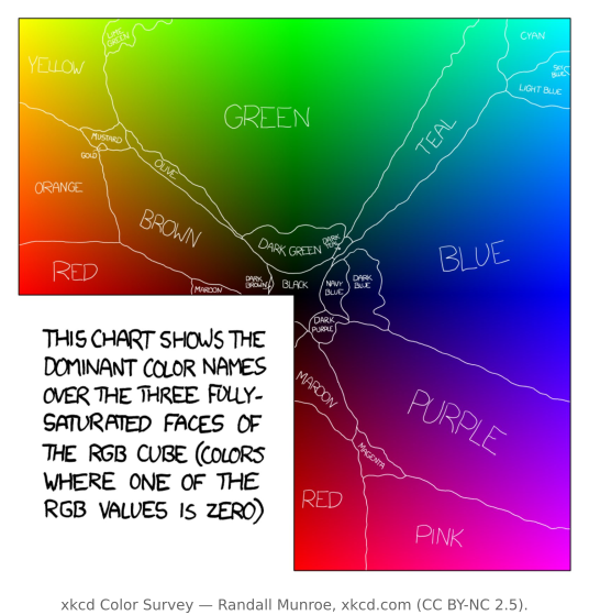
A naming interface benefits from distinguishing a typical example from a boundary. A swatch near a focal red can receive a high probability for “red,” while a swatch between red and orange can receive substantial probability for both. Moving across the model's decision boundary need not create a large perceptual change. A hard label is useful when selecting a menu category, but probabilities are more informative when retrieving images or explaining an ambiguous match. This is the practical meaning of treating a color name as a prototype with a falloff rather than a physical partition of light.
The sequence from spectrum to color name explains why a single set of RGB coordinates cannot answer every color question. Light and surface reflectance determine the incident spectrum; cone responses reduce it to three measurements; adaptation and spatial context affect appearance; naming and memory add categorical and learned associations. These are useful levels of description, not a claim that the brain executes a simple serial software pipeline. A colorimetric match addresses an earlier part of this sequence than a preferred rendering of a familiar face or landscape.
Recap: big lessons of this chapter
YCbCr’s luma is a weighted sum of nonlinear channels. It supports coding and chroma subsampling but is not photometric luminance. Chroma errors can change decoded luminance as well as color. Decode into a defined linear space for a radiometric calculation.
A color-difference magnitude depends on signal scale. In a linear opponent representation, scaling luminance and both centered chroma components together preserves the underlying chromaticity. Ratios describe that algebra, but a ratio such as chroma divided by luminance is not a universal perceptual saturation formula. State what the edit preserves.
$XYZ$, $xy$, RGB, and HSV are built to measure and store color. Judging how different two colors look takes a space deliberately warped for that job, such as CIELAB (CIE 1976 (CIELAB)) with its $\Delta E$. Mixing the two up is why gamut areas on the $xy$ diagram mislead, why a gradient that is even in RGB banks unevenly to the eye, and why an error computed in the wrong space rewards the wrong thing. Ask of any color number: is this for measuring, or for judging?