4.4 RGB color spaces⧉
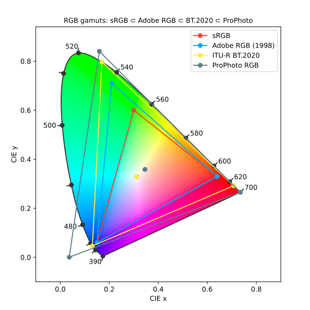
An RGB space chooses primary chromaticities and a reference white; its stored representation also specifies a transfer function. Different choices serve different devices and workflows. sRGB is a common SDR delivery space. Display P3 extends its red and green coverage. Adobe RGB extends especially into greens and cyans useful in some print workflows. Rec. 2020 has still wider primary chromaticities. ProPhoto is a large working space with imaginary primaries.
With fixed integer precision, a larger gamut generally spreads codes more widely in color. The effect varies across the gamut and depends on the transfer function. Use sufficient precision for editing, then choose the delivery space from the output requirements. A screen cannot display every working-space value merely because software can store it.
Choose a working gamut large enough for the content and operations, with sufficient numeric precision. Choose a delivery space the receiving system can interpret. Wider primaries alone do not improve an image, and converting an sRGB image to a wider space does not recover colors previously clipped.
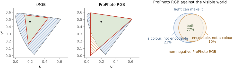
Display-oriented spaces describe a reference set of primaries. Working spaces can instead choose imaginary primaries to enclose more physical colors. ProPhoto’s green and blue are outside the spectral locus; its red is not the imaginary pair’s other member. Such coordinates are useful for calculation, but their nonnegative cube contains values no physical light can produce.
Camera raw is different. Its channels are spectral measurements, often one color sample per photosite in a mosaic, not weights of three emission primaries. A camera would admit an exact universal XYZ matrix if its sensitivities spanned the standard observer’s matching functions. Real cameras generally only approximate this condition, so color correction is fitted and depends on spectra and illumination. It is not meaningful to invert an arbitrary three-by-many sensitivity matrix and call the result three physical display primaries.
Camera profiles can provide multiple illuminant calibrations. Do not assume every DNG contains exactly two matrices at fixed temperatures; use the tags and conventions of the actual profile. Camera color-space menu settings usually govern rendered output and previews, while raw channel interpretation remains camera-specific.
The correction matrix also propagates noise. With equal independent input variances $\sigma^2$, output channel $i$ has variance $\sigma^2\sum_j M_{ij}^2$. More generally use $M\Sigma M^T$. Negative coefficients do not alone prove amplification; their magnitudes and the input covariance matter. The filter design and color fit balance sensitivity, color accuracy, and noise, as developed in Chapter 4.6, Sensing color: multiplexing strategies.
This distinction explains two different kinds of color-conversion experiment. Between linear RGB working spaces built from the same standard observer, convert a color to XYZ and then to the destination coordinates; the two matrices compose into one exact coordinate transform. For a camera, photograph a set of known reflectances under a specified light and fit a matrix from the measured camera responses to their target XYZ values. It can fit those samples well and still make errors on other spectra. Two spectra that the camera records identically cannot be separated by any later matrix, even if the standard observer distinguishes them. More training patches improve the fit over a chosen population; they do not restore spectral information absent from the three measurements.
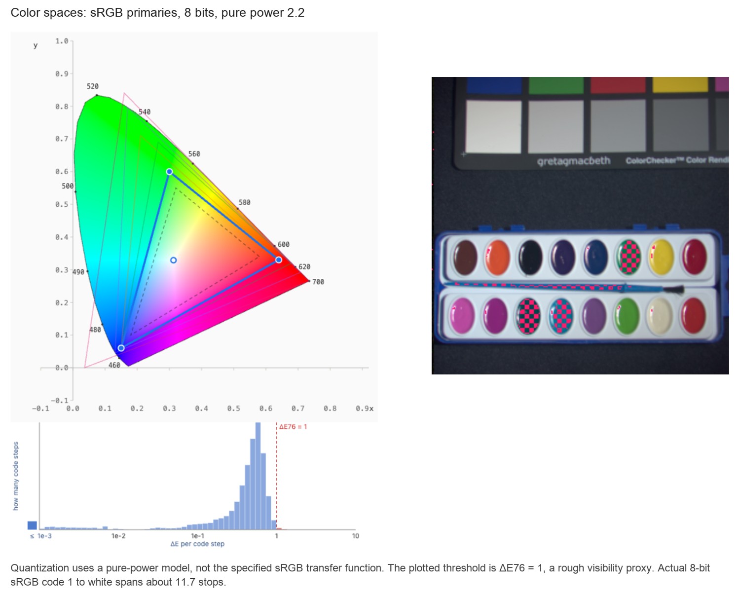
The choice of a working gamut also affects quantization. With a fixed integer bit depth, a wider set of primaries spreads the available code combinations over a larger range of colors. It can retain a saturated color that a smaller space clips, yet give coarser steps in a region shared by both spaces. Increasing bit depth or using floating point reduces that pressure. This is why a space suited to intermediate editing need not be the best choice for compact delivery. The working space must retain the colors the pipeline needs; the output space must match the interpretation supported by the destination.
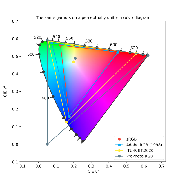
A caution about that diagram before we read too much into the triangle sizes: the $xy$ chromaticity plane is a space for measuring color, not for judging how different two colors look. It stretches the greens enormously and cramps the blues and purples, so neither the relative areas of these gamuts nor the distances between their primaries track perceived difference. Re-plot the identical primaries on a perceptually more uniform diagram, the CIE 1976 UCS ($u'v'$) space, and every triangle changes shape (Figure 4.4.3): the relative areas and distances change. The newer diagram is more uniform, but it is still not a universal perceptual ruler. That $XYZ$ (and its $xy$ projection) is not perceptually uniform is precisely what will force the deliberately non-linear spaces of Chapter 4.5, Advanced color: opponents, perceptually-uniform, and preferred.
Two design processes can lead to an RGB space. In a display-oriented design, begin with the primaries a reference display can emit, then describe colors as amounts of those lights. In a working-space design, begin with the colors that editing should retain, then choose a coordinate system that encloses them. The latter need not correspond to a manufacturable display. An imaginary primary is acceptable as a coordinate axis because no lamp is being asked to emit it while the image is stored or edited. Physical realizability becomes an output constraint when those values are converted for a screen or printer.
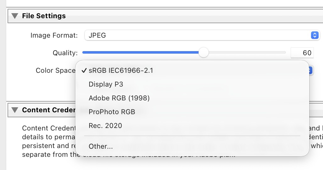
This distinction explains why choosing a larger working space does not upgrade the monitor. It changes which intermediate colors can be represented without clipping to the working cube. Displaying them still requires conversion and, where needed, gamut mapping. Conversely, a delivery space can be chosen for compatibility with the intended viewing path even when a larger space was useful during editing. The export dialog asks for an engineering choice about that destination, not a ranking in which the largest triangle is always best.
The noise formula can be read numerically. A correction row with coefficients 1.8, -0.9, and 0.1 has squared length 4.06. With equal independent input noise, its output standard deviation is therefore about 2.01 times the standard deviation of one input channel. The row may improve the color fit while increasing that channel's noise. This is why a camera characterization should be evaluated for both reconstruction error and noise propagation, using the actual covariance rather than assuming that every color matrix has the same cost.
4.4.1 Two different words for impossible⧉
A chromaticity can be physically realizable yet outside a display’s primary triangle. Conversely, an RGB space with imaginary primaries can encode chromaticities no nonnegative spectrum produces. These are different limitations. Signed floating-point RGB can also represent colors outside its positive-primary triangle, provided subsequent operations preserve the signed values.
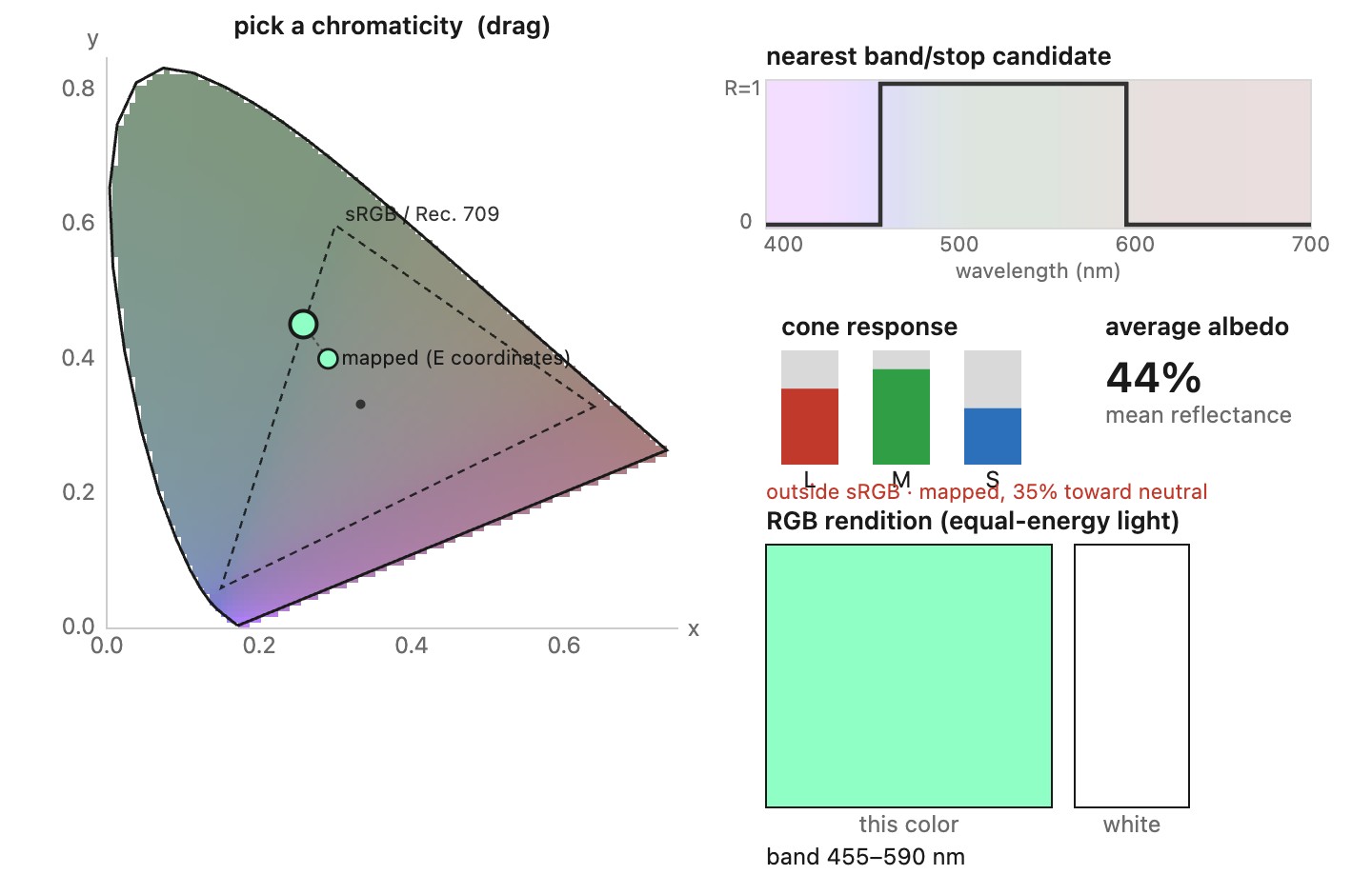
A chromaticity triangle omits luminance. Even a chromaticity inside the triangle may require more light than a display can emit at the requested luminance. Similarly, reflectance is bounded by one: under fixed broadband illumination, pushing a surface color toward a spectral endpoint usually restricts the wavelengths it reflects and reduces its possible luminance. This helps explain the shape of the object-color solid, but does not imply that ordinary pigments always fit sRGB. Saturated flowers, paints, fabrics, structural colors, and colored lights can require gamut mapping.
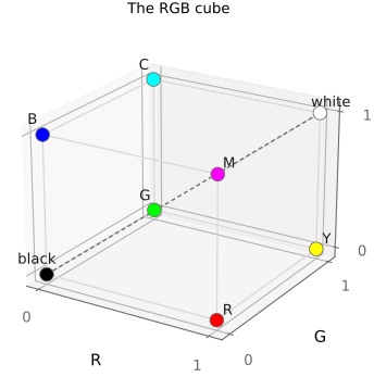
The RGB cube shows the bounded encoding in three dimensions. Its geometry depends on whether its coordinates are linear or nonlinear; its Euclidean distances are not perceptual color differences.
The optimal-reflectance experiment makes the brightness constraint concrete. Under a fixed broadband light, an ideal white reflector returns light across the whole spectrum. Restricting reflection to a narrow wavelength interval rejects the power outside that interval. The resulting chromaticity can be very saturated while the available reflected luminance becomes small. An emitter need not pay this same price: it can put substantial power directly into a narrow band. This is a reason to distinguish surface-color limits from the gamut of colored lights. It does not imply that all colors outside sRGB are nearly monochromatic or that saturated ordinary materials can be ignored.
4.4.2 Reference: primaries, matrices, and transfer functions⧉
Each space named above is fixed by two things: its primaries and white point, which set the linear RGB-to-XYZ matrix, and its transfer function, the gamma curve that encodes the linear values for storage. The matrices below carry linear light, no diacritic, into $\mathrm{XYZ}$; the transfer is applied afterward to get the stored $R'G'B'$ (the primes of Chapter 4.3, Encoding: linear, gamma or log). The middle row of each matrix is that space's luminance $Y$ weighting, the coefficients also used, with the specified nonlinear encoding, to define a corresponding luma (L4.5).
sRGB and Rec. 709 primaries (D65) share this linear matrix, though their transfer conventions differ:
sRGB transfer: piecewise, a linear segment $R' = 12.92\,R$ for $R \le 0.0031308$ splicing into $R' = 1.055\,R^{1/2.4} - 0.055$, overall close to $\gamma = 2.2$.
Adobe RGB (1998) (D65), wider greens for print work:
Transfer: a pure power law, $\gamma = 2.19921875$ (that is $563/256$).
Display P3 (D65), the DCI-P3 primaries on the sRGB white:
Transfer: the sRGB piecewise curve.
ITU-R BT.2020 / Rec. 2020 (D65), ultra-high-definition with very wide primaries (its red is a near-monochromatic 630 nm):
Transfer: BT.2020 specifies a camera-side piecewise encoding with a 0.45-power segment and linear toe. Specify the display response separately. Rec. 2100 uses the same primary chromaticities with PQ or HLG HDR systems (Chapter 4.3, Encoding: linear, gamma or log).
ProPhoto RGB (ROMM) (white point D50), a large editing space with imaginary green and blue primaries:
Transfer: $\gamma = 1.8$, with a short linear segment (slope $16$) below $R = 1/512$.
Two reminders the type system enforces. The matrices are all defined on linear light, so a conversion between two of these spaces is $M_2^{-1} M_1$ applied to linear RGB, never to the stored $R'G'B'$: decode first. And the white points are not all the same (ProPhoto is D50, the rest D65), so a white-relative ProPhoto-to-sRGB conversion includes chromatic adaptation (often Bradford, Chapter 4.2, White balance and white point) between the XYZ stages. A stimulus-preserving conversion has a different objective and does not silently adapt the white.
For a white-relative conversion, the full order is
linear_source = decode_source(encoded_source)
XYZ_source = M_source @ linear_source
XYZ_target = adapt_white(XYZ_source, source_white, target_white)
linear_target = solve(M_target, XYZ_target)
# Retain extended range while working; map gamut for the chosen output.
encoded_target = encode_target(mapped_linear_target)
The printed matrices are rounded reference values. Use a consistent precision and white normalization in code. Verify that RGB white maps to the stated XYZ white and that an unmodified in-gamut round trip returns its input.
Recap: big lessons of this chapter
Choose a working gamut large enough for the content and operations, with sufficient numeric precision. Choose a delivery space the receiving system can interpret. Wider primaries alone do not improve an image, and converting an sRGB image to a wider space does not recover colors previously clipped.