3.4 Spatial and temporal vision🔗⧉

Move a photograph farther away and fine texture becomes harder to see. Increase its contrast and some texture reappears. Visibility depends on angular size and contrast, as well as luminance, color, motion, and where we look. These dependencies help choose display resolution and compression settings.

3.4.1 Spatial vision🔗⧉

How fine a pattern can we resolve, and how does sensitivity vary with the scale of the detail? Visual acuity (the familiar eye-chart measure) sets the finest line spacing we can make out, but it is only the high-frequency tail of a larger story.

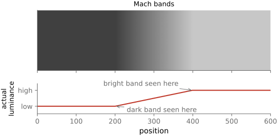
Many retinal neurons have center–surround receptive fields, comparing signals over neighboring regions. Such models can produce edge overshoots resembling Mach bands Mach 1865 (Mach bands) (Figure 3.4.1⛶ fullscreen). They illustrate one contribution to spatial processing; no single lateral-inhibition filter explains every lightness illusion.

A contrast sensitivity function (CSF) describes detection thresholds for specified stimuli, often sinusoidal gratings. Sensitivity is the reciprocal of threshold contrast. Under common photopic conditions, luminance sensitivity is band-pass: intermediate spatial frequencies are easier to detect than very coarse or very fine gratings. The curve changes with viewing conditions.

This experiment can be reproduced directly (Figure 3.4.2⛶ fullscreen). In the Campbell–Robson chart Campbell & Robson 1968, spatial frequency rises to the right and contrast rises downward, the same contrast range in every column, yet the height at which the stripes fade into flat gray is an inverted U, not a level line. The visibility boundary traces the observer's contrast sensitivity function. And because the CSF is measured in cycles per degree of visual angle, the boundary moves with viewing distance: step back and the fine bars on the right vanish first.

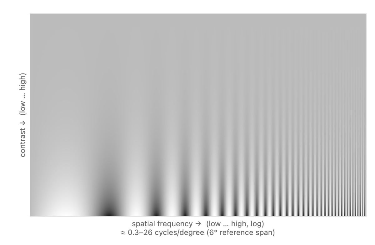
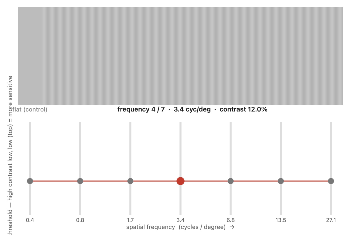
Figure 3.4.3⛶ fullscreen lets you adjust grating contrasts at several spatial frequencies. It illustrates a method-of-adjustment experiment. The display transfer function, ambient reflections, pixel sampling, and quantization affect the result; sRGB encoding and dithering alone do not calibrate an arbitrary screen.

The Mannos–Sakrison fit provides a compact relative frequency weighting Mannos & Sakrison 1974:

Here $f$ is spatial frequency in cycles per degree. The curve peaks near 8 cycles/degree. It has no hard high-frequency cutoff and is not, by itself, a calibrated absolute detection threshold for the reader. Its value at zero frequency should not be interpreted as a universal ability to detect a uniform field change. Evaluated, it gives relative weights of about 0.32 at 1 cycle/degree, 0.98 near the 8 cycle/degree peak, 0.19 at 30 and 0.004 at 60: an error pattern at 30 cycles/degree counts about a fifth as much as the same pattern near the peak, and one at 60 barely counts at all.

Convert image frequency to angular frequency before using such a model. For a centered display of width $w$ viewed at distance $d$, the horizontal angular span is

A pattern with $m$ cycles across that width has average frequency $f=m/\theta$. For example, 30 cycles across 10 degrees gives 3 cycles/degree. This average is a useful small-field approximation; a wide perspective display needs the local pixel-to-angle mapping.

A more complete luminance model also accounts for the light level and the size of the test. Barten's work Barten 1999 is an important example, with applications to display encoding. The compact Mannos–Sakrison curve is useful when a relative weighting by spatial frequency is enough; it should not silently replace the richer conditions of an absolute visibility prediction. This is the engineering purpose of a CSF: errors at different angular frequencies need not receive the same weight.

3.4.2 Chrominance spatial vision🔗⧉

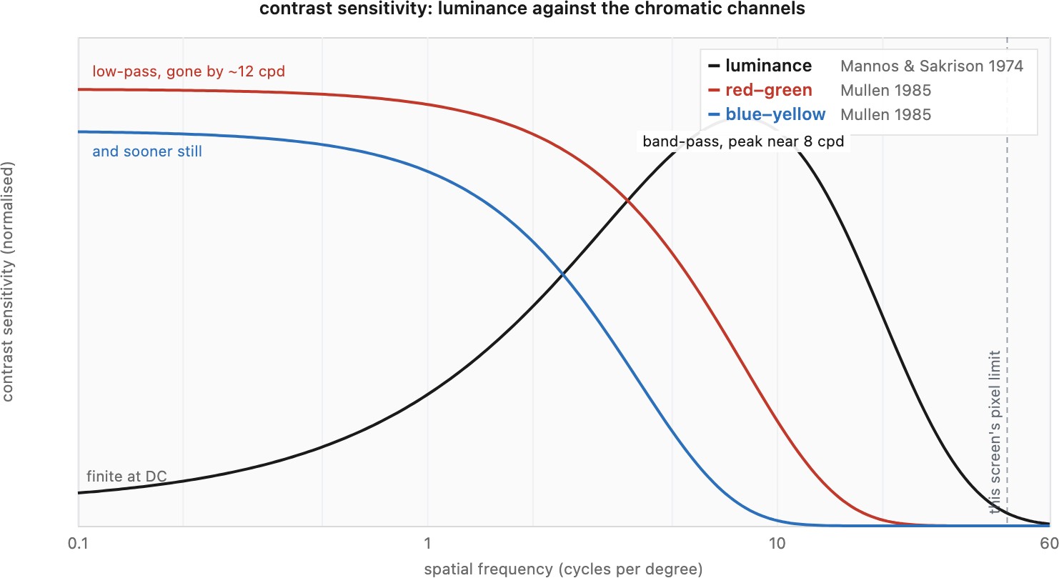
Chromatic gratings can have lower high-frequency sensitivity than luminance gratings Mullen 1985 (Figure 3.4.4⛶ fullscreen). Their apparent sensitivity depends on how cone contrast is normalized and how well luminance artifacts are eliminated. A generic RGB red–green pattern on an uncalibrated screen does not isolate a physiological opponent mechanism.

Reducing chroma resolution often preserves apparent sharpness in photographs. It can also produce bleeding around colored lettering or isoluminant boundaries. JPEG and video encodings exploit the statistical and perceptual benefits, with a tradeoff that depends on the image and output scale. Engineering luma is distinct from physical luminance.

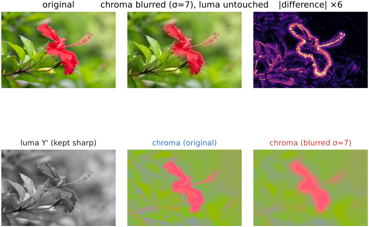
Optics, receptor sampling, and neural processing all affect spatial sensitivity. Sparse S-cone sampling is one limit on short-wavelength chromatic detail. Taking a difference between cone responses is not itself spatial low-pass filtering; the receptive fields and subsequent processing matter. The measured CSFs, rather than a sum-and-difference matrix alone, support decisions about chroma resolution.

Try the bandwidth difference directly. Convert a photograph to a luma–chroma representation, keep the luma unchanged, and blur only chroma. Compare that result with one in which only luma is blurred. Many ordinary photographs retain much more apparent detail in the first case. Saturated small text and sharp color boundaries can still reveal the chroma blur. This experiment explains both the attraction of chroma subsampling in JPEG and video and an important failure case: the visibility depends on the image content and viewing conditions, not only on the number of samples removed.

3.4.3 Temporal vision🔗⧉

A flashing source can appear steady when modulation becomes too fast to detect. The threshold depends on luminance, modulation depth, area, retinal location, waveform, and the observer. There is no universal 60 Hz limit. Peripheral flicker sensitivity under bright conditions cannot be explained by rod density alone; cones support faster responses than rods.

Temporal modulation and sampled motion are different tests. A sample-and-hold display may show no visible flicker yet blur moving detail as the eye tracks it. A projector can flash each film frame more than once to reduce flicker without increasing the number of distinct motion samples. Frame rate, refresh rate, illumination pulses, and exposure duration must therefore be specified separately.

Models such as stelaCSF and castleCSF combine spatial and temporal frequency with adaptation and viewing geometry Mantiuk et al. 2022 Ashraf & Mantiuk 2024. Rather than replacing the published model with a separable product, use its reference implementation. Abstractly, its output is

The inputs describe spatial frequency, temporal frequency, adapting luminance, eccentricity, stimulus area, and color-modulation direction. The threshold contrast uses the model's contrast convention. A luminance grating and a chromatic grating cannot be compared by feeding unrelated RGB amplitudes into this equation.

conditions = calibrated viewing geometry and adapting luminance
stimulus = angular frequencies, area, eccentricity, color direction
sensitivity = published_CSF_model(conditions, stimulus)
threshold = 1 / sensitivity
compare stimulus contrast in the model's units with threshold

This predicts thresholds within the model's tested domain. Natural-image masking, attention, and suprathreshold appearance require more than an isolated-grating threshold. The castleCSF reference code provides the model versions and input conventions.

Apparent motion allows successive images to be perceived as movement Wertheimer 1912 (phi phenomenon); it should not be reduced to a retinal afterimage or “persistence of vision.” Eye movements, exposure blur, and display timing all affect the result. These distinctions matter when choosing capture rates or amplifying small temporal changes (Chapter 38.3, Motion and video magnification).

The input list describes concrete experiments. Keep the grating fixed and increase the background luminance: its threshold changes. Move the same pattern away from fixation: fine detail usually becomes harder to detect. Increase its area: more cycles can contribute evidence, up to limits imposed by spatial summation. Change the flicker rate while also changing stripe spacing: spatial and temporal sensitivity interact, so two independently chosen one-dimensional curves need not predict the result.

Classical temporal models describe sustained and transient responses using filters with different time constants Watson 1986. A slow response follows gradual changes; a faster response makes brief changes more visible. Combining them can produce a band-pass frequency response. The published models specify how those responses depend on the stimulus and how they are combined. Those dependencies, and the fitted constants, are part of the model rather than arbitrary tuning knobs. They explain why the model interface needs more information than a frame rate.

Recap: big lessons of this chapter🔗

💡 Big lesson (L3.14) — contrast sensitivity is frequency-tuned, and it lives per degree🔗

The eye is not equally sensitive to every spatial frequency. Luminance sensitivity is band-pass, peaking at a few cycles per degree and falling away on both sides, and the curve moves with light level, field size and contrast. It is defined per degree of visual angle, not per pixel, so viewing distance and display size decide which frequencies a reader can resolve at all. Quote a peak from a textbook and you have described one experiment's conditions; measure it in the conditions you ship in.

💡 Big lesson (L3.15) — chrominance resolves less than luminance🔗

The chromatic contrast-sensitivity functions are low-pass where the luminance one is band-pass, and they cut off at a far lower frequency, so fine color variation is much less visible than fine luminance variation. Chroma subsampling is the engineering that spends that gap. It describes typical content under typical viewing, not a law: colored lettering, isoluminant boundaries and saturated fine patterns can make the loss plain. Judge it on the content you actually have, in the viewing conditions you actually ship.

💡 Big lesson (L3.16) — chromatic acuity depends on sampling and processing🔗

Spatial sensitivity depends on optics, receptor sampling, and neural processing. Chromatic detail often supports less resolution than luminance detail, but this cannot be deduced from opponent subtraction alone. Use measured sensitivity and inspect the intended images.

💡 Big lesson (L3.17) — vision has a finite temporal bandwidth🔗

Temporal visibility depends on stimulus and viewing conditions. Flicker fusion does not determine a universal frame rate for smooth motion. Distinguish exposure duration, distinct image samples, display refresh, and light modulation when designing or evaluating video.

💡 Big lesson (L3.18) — low-level perception is quantitative: it has analytic models you can evaluate🔗

Psychophysical models make quantitative predictions for specified tasks and conditions. Use the documented stimulus units, calibration, and validity range. A predicted detection threshold is not a guarantee that an arbitrary image artifact will be invisible.