3.3 Adaptation and constancy⧉
A white page can remain recognizable as white when moved into shadow, even though it sends less light to the eye. Adaptation adjusts sensitivity to the prevailing light; constancy supports relatively stable judgments about surfaces. Neither removes all effects of illumination. The distinction matters when choosing the exposure and rendering of a photograph.
3.3.1 Light adaptation⧉
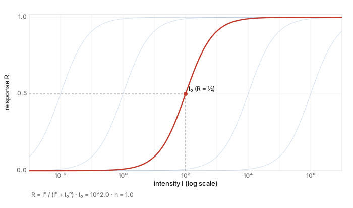
Walk into a dark cinema and details gradually become visible. The visual system changes sensitivity as the prevailing light changes. A useful model of a saturating response is the normalized Naka–Rushton curve Naka & Rushton 1966,
At intensity $I=I_0$, the response is one half. Changing $I_0$ moves the operating range; $n>0$ controls the slope. This family can describe measured responses, but one curve and a moving average do not specify all of light adaptation. The curve is sigmoid when plotted against log intensity; for $n=1$ on linear axes it is a saturating hyperbola.
Figure 3.3.1 lets you change the operating point and compare axis scales.
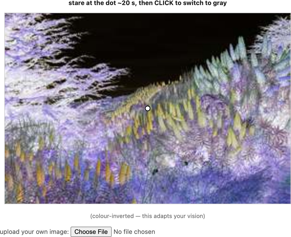
Neural gain control, photopigment bleaching and regeneration, and pupil changes contribute on different timescales. A pupil diameter change from 2 to 7 mm changes area by $(7/2)^2\approx12$, much less than the full range over which vision operates. Full dark adaptation can take tens of minutes. Local adaptation also contributes to afterimages. In the Spanish-Castle demonstration, an adapting color image is followed by a grayscale version that briefly appears colored (Figure 3.3.3); the effect is not an illusion of motion.
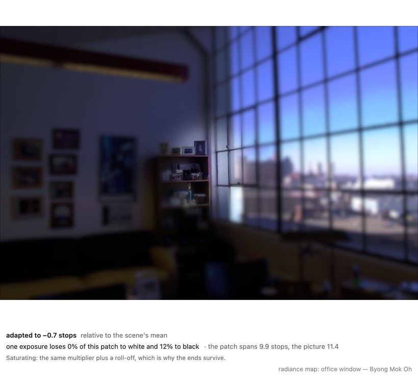
Distinguish sensitivity across adaptation states from the range visible in one scene under specified conditions. Local adaptation, glare, spatial structure, and the task all affect that range. A single stop count is insufficient to compare an eye, camera, and display.
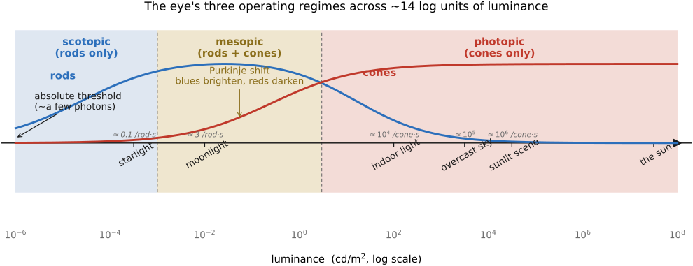
Vision is often described in three regimes. Photopic vision is cone-dominated and supports detailed color vision. Scotopic vision is rod-dominated and lacks ordinary trichromatic color discrimination. Mesopic vision combines rod and cone signals. The transitions depend on adaptation, spectrum, retinal position, and stimulus, so they are not universal luminance cutoffs.
As illumination falls, relative spectral sensitivity shifts toward shorter wavelengths, the Purkinje shift Purkyně 1825 (Purkinje shift). A red flower can become relatively darker than nearby blue-green foliage. This is a change in relative sensitivity, not a statement that all dim scenes look blue. Luminance (cd/m²) describes light from a surface in a viewing direction; illuminance (lux) describes light arriving at a surface. A scene's lux value alone does not determine the observer's adaptation state.
Retinal illuminance is often summarized in trolands: luminance in cd/m² multiplied by pupil area in mm²,
For example, a 100 cd/m² patch viewed through a 3 mm diameter pupil gives about $100\pi(1.5)^2\approx707$ trolands. This is a photometric convention, not a universal conversion to photons. For order of magnitude only, Rodieck's estimates put a rod under starlight at roughly one photoisomerization every several seconds, and a cone in a sunlit scene at around a million per second Rodieck, The First Steps in Seeing, a span the pupil, bleaching and neural gain together have to accommodate. Predicting photoisomerizations additionally requires the spectrum, ocular transmission, receptor sensitivity and collecting area, and integration time. A photon absorbed by a visual pigment can isomerize the molecule and initiate a graded receptor response; it does not necessarily cause a perceptible event.
At very low light levels, photon statistics and neural noise limit detection. Hecht, Shlaer, and Pirenne inferred that a detectable flash could produce only a few photoisomerizations distributed across many rods Hecht, Shlaer & Pirenne 1942. Recordings subsequently established that individual rods can respond to single photons Rieke & Baylor 1998. That cellular response must be distinguished from conscious detection. Tinsley and colleagues reported slightly above-chance detection of single photons incident on the cornea Tinsley et al. 2016 (humans detect a single photon), but later retinal and psychophysical work challenged the interpretation of that result (2024 study). These findings do not make the eye a reliable photon counter. Chapter 2.8, Noise, signal-to-noise ratio and dynamic range explains the corresponding photon-counting limits in cameras.
The range over which we can function after adapting is much greater than the range we can distinguish at one operating point. A bright scene and a dark cinema do not both fit into one unchanged receptor response. Adaptation moves that response so its useful slope falls near the current stimulus levels. This is why a claim about the eye's total dynamic range does not specify how many stops a display must reproduce simultaneously. HDR capture and tone mapping must account for the scene, the display, and the observer's adaptation separately.
3.3.2 Visual perception is largely invariant to multiplications⧉
A cloud can reduce the light on a page while leaving its print recognizably black on white. Ratios between surface luminances can remain unchanged even though the overall scene looks dimmer. This approximate stability concerns surface appearance and discrimination; it does not mean the observer cannot detect a change in illumination.
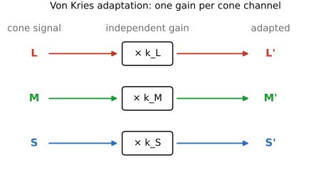
The mechanism is gain control, and gain control is multiplication. A photoreceptor in a bright field turns its sensitivity down, one in dim light turns it up, and each does so, to a first approximation, by scaling its response by a factor set by the local average. Chromatic adaptation is the same operation run channel by channel: the von Kries model is an independent multiplicative gain on each cone class, the diagonal model we use for white balance. Light adaptation, from the previous section, is its achromatic version.
In a simple matte-surface model, luminance is proportional to illumination times reflectance. Ratios between nearby surfaces cancel a shared illumination factor. Shadows, interreflections, specular reflection, and different surface orientations can violate that shared-factor assumption. Local gain control helps explain some stability, while spatial organization and interpretation supply other cues.
Changing exposure time or aperture scales the expected sensor signal within the linear, unclipped regime. ISO changes gain and camera behavior; it does not itself increase the photons captured. Exposure is measured in stops because a stop corresponds to a factor of two. These multiplicative descriptions are useful for processing, but changing exposure does not reproduce visual adaptation.
The experimental record is old and specific. Wallach showed that the perceived lightness of a disk is fixed by the ratio of its luminance to its surround: hold that ratio and the gray looks the same through a hundredfold change in absolute light Wallach 1948 (ratio principle). Land and McCann built Retinex on the same principle, computing lightness from ratios taken along spatial paths so that slow illumination gradients fall away Land & McCann 1971. Gilchrist's Seeing Black and White gathers decades of such findings into an account of how vision anchors lightness and assigns it across a scene Gilchrist 2006 (Seeing Black and White).
The stability is partial and task-dependent. Surface-lightness matches can remain relatively constant where brightness matches change Arend & Goldstein 1987. Constancy also depends on available scene cues Kraft & Brainard 1999. At low light levels, photon and neural noise, receptor changes, and threshold behavior limit a simple gain model.
A ratio can be invariant to a common scale without any logarithm. For positive $I$ and a positive local estimate $B$, scaling both by $\alpha>0$ leaves $I/B$ unchanged. A logarithm represents the same ratio as a difference:
The offset introduced by scaling cancels in the difference. The individual log values change, so log encoding is not itself invariant. Divisive normalization and logarithmic coordinates are related mathematical tools, not interchangeable claims about neural implementation.
A stored HDR image can use linear floating point, log encoding, or another transfer function. Log values make exposure changes additive and provide approximately relative precision over positive values. They are useful, not mandatory. Encoding choice must also handle zero, negative intermediates, quantization, and the operations to be performed (Chapter 4.3, Encoding: linear, gamma or log).
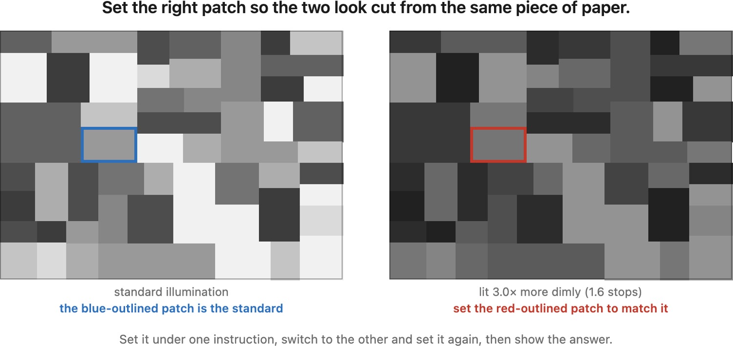
Shared multiplicative changes preserve ratios and often leave surface appearance approximately stable. Brightness, visibility, and color can still change. Gain-control models are useful within their assumptions; they do not make vision insensitive to illumination.
Dividing a value by a similarly scaled reference cancels a common multiplier. Taking logarithms turns the ratio into a difference. This explains why log coordinates are useful for relative changes, without claiming that vision uses a global logarithm or that HDR storage requires one.
Consider two matte patches side by side under the same illumination. In a scalar illumination–reflectance model, doubling the illumination doubles both luminances, but leaves their ratio unchanged. That ratio therefore carries information about the relative surface reflectances without requiring the observer to know the illumination level. Put one patch into a cast shadow and the cancellation no longer holds: the two patches now have different illumination factors. The visual system needs spatial context to decide whether a change is a material boundary or a lighting boundary. This is the connection between multiplicative image formation, ratio-based descriptions of contrast, and the harder inference problem of constancy.
3.3.3 Contrast⧉
If vision reads ratios, its natural unit is contrast, and the oldest quantitative statement of that is Weber's law (Weber 1834 (Weber's law)): the just-noticeable increment in intensity is a roughly constant fraction of the background, $\Delta I / I \approx \text{const}$. The smallest brightness change you can detect grows in proportion to the brightness already there. A candle added to one candle is obvious; the same candle added to a hundred is nothing.
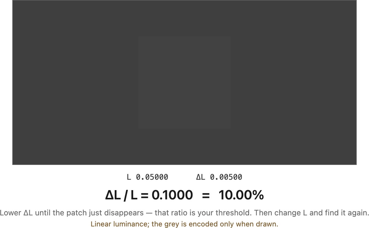
Weber's law is a statement about threshold. It describes the smallest increment you can just detect, and there it holds well across the middle of the photopic range, but it says nothing about how strong a large, plainly visible contrast looks. That suprathreshold regime has its own accounts, and two classical ones matter here. Fechner integrated Weber's law, treating each just-noticeable difference as one equal step of sensation, and reached a logarithmic relation between intensity and perceived magnitude, $\psi \approx k \log \phi$ Fechner 1860 (Elemente der Psychophysik). Stevens, from direct magnitude estimation, argued instead for a power law, $\psi = k\,\phi^{a}$, with an exponent that depends on the modality Stevens 1957 (power law). Which is right has been argued for a century and does not need settling here.
These models preserve different relations. A common scale leaves Weber contrast unchanged. Under Fechner's model it adds a constant to perceived magnitude, preserving differences; under Stevens's model it scales magnitude, preserving ratios. Neither implies unchanged brightness. Gamma encoding is a power law and does not turn a multiplier into an additive offset; a logarithm does.
For a small target on a uniform positive background $L_b$, use Weber contrast. For a periodic grating, use Michelson contrast:
The first measures a target's increment or decrement relative to its background. The second measures modulation relative to the midpoint of a periodic pattern's extrema. Both cancel a common positive multiplier, but they describe different stimuli. For luminances 80 and 120, Michelson contrast is 0.2; a 120 target on an 80 background has Weber contrast 0.5. Use linear luminance, not encoded pixel values.
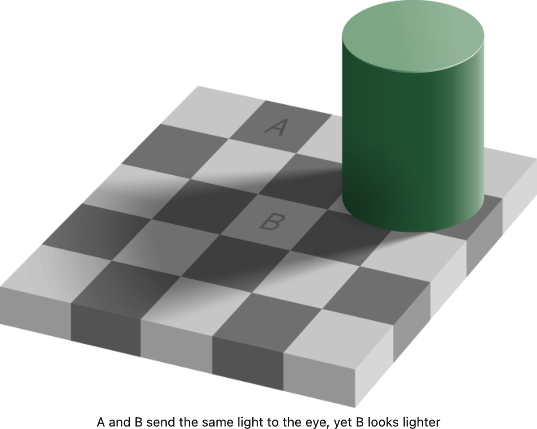
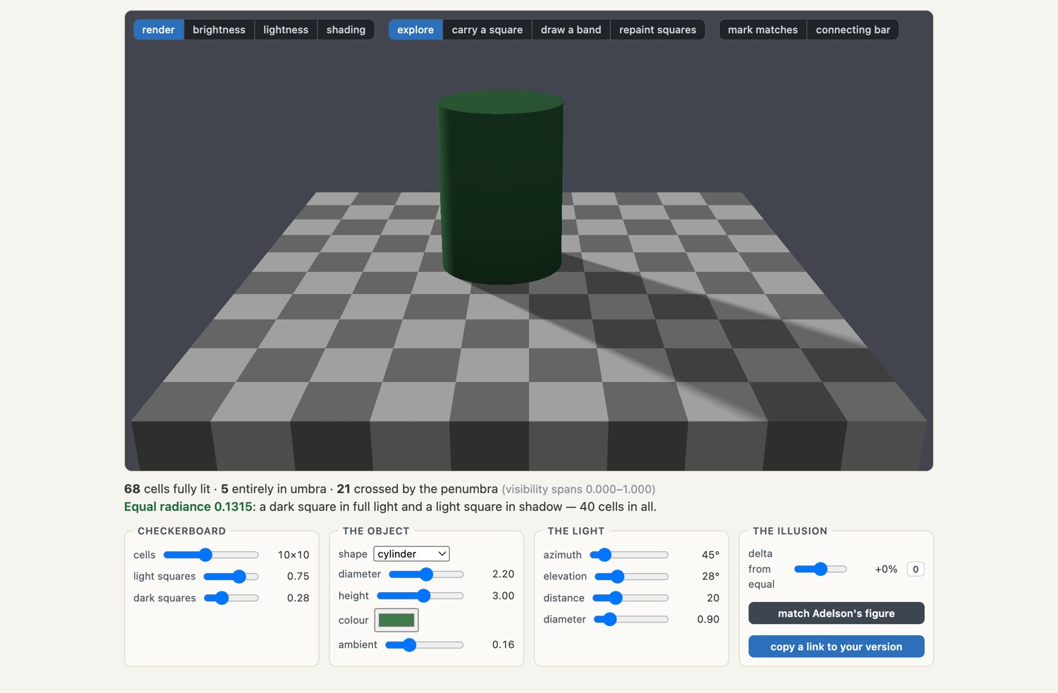
Contrast is set by context too, not by a patch in isolation. A gray patch looks lighter on a dark surround and darker on a light one, the effect called simultaneous contrast (Chevreul 1839 (simultaneous contrast)), while the Adelson checker-shadow illusion adds cues about scene geometry and illumination. Meet it in its barest form before any tone-mapping operator arrives, because every one of them is a machine for changing exactly this (Figure 3.3.7).
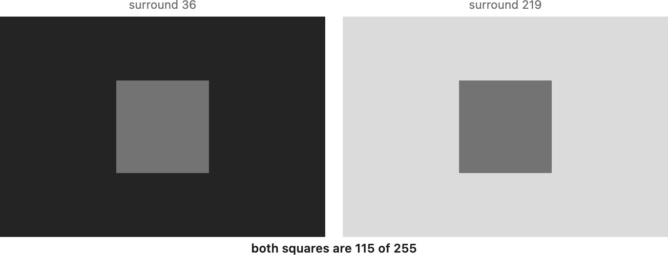
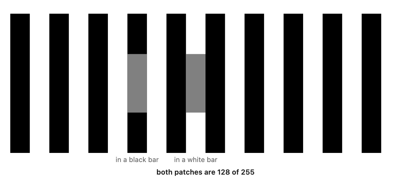
That much is compatible with a simple story: the response to a patch is divided by the light around it, so more surround means a darker-looking patch. Simple surround averaging cannot account for White’s illusion (Figure 3.3.8), which is a counterexample to simple surround division: the patch that looks lighter is the one with more white against it, which is the opposite of what dividing by the surround predicts. Perceptual grouping and junction structure contribute beyond immediate border contrast.
Detectable increments often scale approximately with the background in the photopic range. State which contrast definition, stimulus, and viewing conditions a measurement uses. Absolute pixel error and perceived difference answer different questions; neither replaces the other.
3.3.4 Lightness constancy⧉
A white page in shadow can look lighter in surface color than sunlit coal even if the coal sends more light to the eye. Lightness is perceived surface reflectance; brightness is the perceived amount of light. Lightness constancy is approximate stability of the former as illumination changes. It is not exact recovery of physical reflectance.
In the simple product model, separating illumination and reflectance from one image is underdetermined. Vision uses context, edges, spatial organization, and prior experience. A sharp edge can be a reflectance boundary or a shadow; a smooth variation can be illumination or a surface pattern. No rule that classifies edges by sharpness alone solves the problem.
Adelson's checker-shadow illusion shows two equal pixel values that appear to belong to different surface lightnesses Adelson 2000 (Figure 3.3.9; source explanation). Shadow cues and local relationships support different interpretations of the two squares. Retinex models use spatial comparisons to estimate lightness Land & McCann 1971, and intrinsic-image methods explicitly separate reflectance and shading. These are models of the inference, not established descriptions of a single neural algorithm.
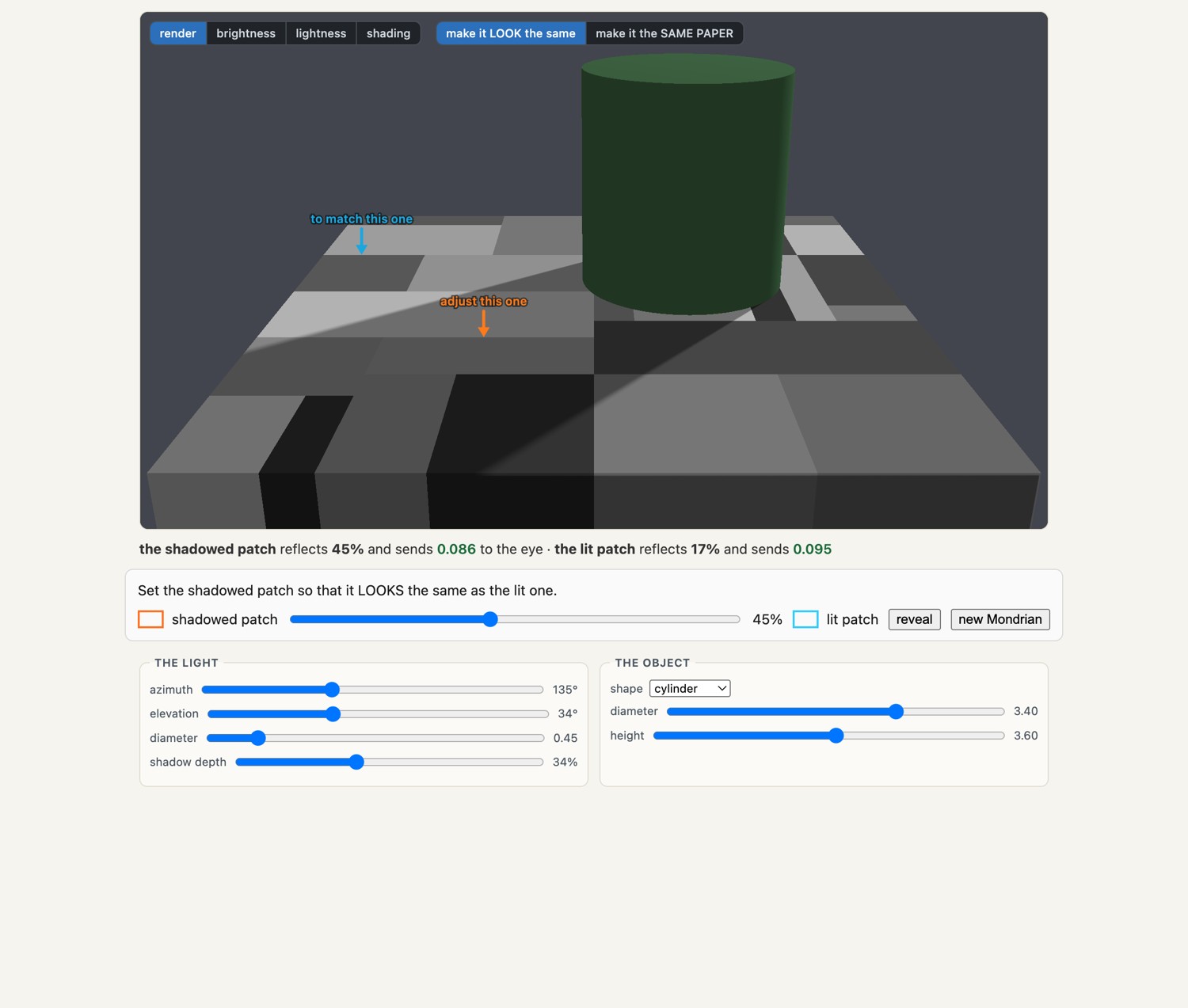
The Gelb effect illustrates the importance of context Gelb 1929 (the Gelb effect). A black paper illuminated by a hidden spotlight in a dark surround can appear white. Adding a white reference can make it appear darker. The result depends on how the visible surfaces are grouped and interpreted; it does not establish perfect constancy in ordinary scenes.
The Moon provides a familiar comparison. Its average reflectance is low, yet against a dark sky it can appear bright and nearly white. Brightness and surface lightness are different judgments: strong illumination can make a dark material bright. Images containing both Earth and Moon help compare their reflected light (Figure 3.3.13), although exposure, geometry, and rendering also affect the photograph.

Estimating stable surface properties helps recognize materials across lighting changes. Illumination is also useful information: it describes shadows, shape, weather, and time of day. Vision does not simply discard it, and a photographer may choose to emphasize it.
Surface-lightness and color judgments can remain relatively stable as illumination changes. This constancy is partial and uses several cues. It differs from recovering the complete reflectance spectrum, and it does not imply that brightness or the appearance of lighting stays fixed.
An incident-light meter or a known gray reference helps choose an exposure without mistaking a dark subject for weak illumination. Their use does not guarantee the same rendering in all conditions: orientation, lighting variation, meter calibration, and clipping still matter (Chapter 5.2, Exposure and capture timing).
Lighting can be the subject of a photograph. A long cast shadow records the direction of sunlight; a caustic on a nearly uniform cloth records how glass redirects it (Figure 3.3.14). The print represents those variations as ink reflectance, while a display represents them as emitted light. The viewer can still interpret them as illumination in the depicted scene.

A photographer can deliberately make illumination the subject. On a nearly uniform white cloth, a glass casts a caustic whose structure comes mainly from the redirected light rather than a change of material. A low sun can make a person's shadow a stronger graphic shape than the person. Printing the photograph fixes those variations as different ink reflectances, so the pattern can be examined under new lighting long after the original caustic or shadow has disappeared. This does not prevent the viewer from recognizing depicted illumination; it separates the light on the print from the light represented by the print (Figure 3.3.14).
The metering connection is concrete. A reflected-light meter cannot tell whether a weak signal came from low illumination or a dark subject. Measuring a gray card of known reflectance under the subject's light removes one unknown from that comparison. An incident meter measures the arriving illumination instead of relying on the subject's reflectance. Both approaches help avoid brightening a black subject merely because it is black. They still require representative lighting and an exposure compatible with the range the camera can capture.
3.3.5 Color constancy⧉
Discounting the illuminant⧉
A white shirt can remain recognizably white under daylight or a warm lamp despite a change in the spectrum reaching the eye. Color constancy describes this approximate stability of surface-color judgments. It does not imply recovery of the surface's full reflectance spectrum. Illuminant estimation, adaptation, and spatial context all contribute.
Von Kries adaptation models an independent gain on each cone class Von Kries (Figure 3.3.16). Gains chosen to map an adapting white to a reference white give a useful approximation, not exact illuminant removal for every surface. Chapter 4.2, White balance and white point develops the corresponding transform and its limits.
Camera white balance estimates gains or a more general transform to render the scene for the intended output. Gray-world, bright-pixel, and learned methods use different evidence. These engineering estimators need not duplicate the visual system's computation Freeman & Brainard (Bayesian color constancy).
In low light, weak cone signals and increased rod contributions reduce color discrimination. A camera that accumulates a burst may record color that was difficult to see during capture. Night Sight uses learned white balance as part of a pipeline demonstrated down to 0.3 lux Liba et al. 2019. That illuminance is a capture condition, not a universal threshold below which no person has useful color information. The desired rendering may also preserve some warmth or darkness rather than fully neutralizing the scene.
Chromatic adaptation and scene interpretation help stabilize surface color across illuminants. Per-channel cone gains are a useful approximation. Camera white balance makes a related rendering choice for the output conditions, with accuracy limited by the measurements and estimated illuminant.
Failure of color constancy when viewing photographs⧉
A photograph supplies cues about a depicted scene while also being an object viewed under different conditions. The display white, room lighting, image content, viewing angle, and adaptation state can all influence its appearance. A tungsten-lit scene on a daylight-balanced display may therefore look more orange than the scene did during capture. White balance helps choose the intended relationship between capture and viewing conditions; it need not remove every visible trace of the illuminant.
Experiments show that constancy depends on scene cues and on what observers are asked to match Kraft & Brainard 1999 Arend & Reeves 1986 Brainard et al. 2006 (Bayesian human constancy). Displayed images can support substantial constancy when they supply useful cues. A photograph does not switch that ability off. Color-appearance models describe effects of specified viewing conditions, but should not be confused with ICC rendering intents or a complete account of scene interpretation Fairchild, Color Appearance Models.
There is also a measurement limit. Two surface spectra can produce the same camera channels under one illuminant and different responses under another. No deterministic mapping of that single triple can separate the surfaces. White balance cannot reconstruct wavelengths that the illumination did not supply. This matters with narrowband sources and is distinct from a viewer's incomplete adaptation (Chapter 3.2, Perceptual color and trichromatic vision).
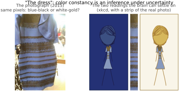
The 2015 photograph of “the dress” demonstrates that viewers can interpret the same displayed image differently Lafer-Sousa et al. 2015 (Figure 3.3.17). Assumptions about illumination contribute to the blue-black and white-gold reports. The effect supports the role of inference under ambiguous conditions; it does not prove that two simple illuminant choices fully explain every observer's response.
A photograph is viewed under conditions different from those at capture. Its appearance depends on the display or print, the surround, adaptation, and cues within the picture. White balance and rendering should target those conditions and the photographer's intent; viewers do not automatically undo the captured illuminant.
A print has two illumination contexts. Light in the room falls on the paper; within the image, shadows and highlights depict light that fell on the original scene. The viewer can recognize both, but they need not support the same adapting white. This is the dual character of picture perception discussed by Mausfeld Mausfeld 2003 (dual code). It explains why simply reproducing the captured color coordinates need not reproduce the appearance experienced by the photographer.
For example, consider a white wall photographed under a warm lamp and shown on a display in a daylight-lit room. The camera measured the warm spectrum reflected by the wall. Displaying that cast unchanged can make the wall appear more orange than it did to someone adapted to the original room. White balance supplies a rendering decision about that difference. Neutralizing every surface is not compulsory: the photographer may want the warmth of the lamp to remain. The distinction is between a measurement of the light that arrived and a choice about how the scene should look under new viewing conditions.
The inference is difficult because the camera did not separately measure illumination and reflectance. A correction toward a reference illuminant uses assumptions about the source and the surfaces. If the source supplied almost no energy in some wavelength range, the photograph contains little evidence about reflectance there. A plausible correction cannot manufacture that evidence. This connects the perceptual motivation for white balance to the spectral measurement limits developed in the color part.
Recap: big lessons of this chapter
Distinguish sensitivity across adaptation states from the range visible in one scene under specified conditions. Local adaptation, glare, spatial structure, and the task all affect that range. A single stop count is insufficient to compare an eye, camera, and display.
Shared multiplicative changes preserve ratios and often leave surface appearance approximately stable. Brightness, visibility, and color can still change. Gain-control models are useful within their assumptions; they do not make vision insensitive to illumination.
Dividing a value by a similarly scaled reference cancels a common multiplier. Taking logarithms turns the ratio into a difference. This explains why log coordinates are useful for relative changes, without claiming that vision uses a global logarithm or that HDR storage requires one.
Detectable increments often scale approximately with the background in the photopic range. State which contrast definition, stimulus, and viewing conditions a measurement uses. Absolute pixel error and perceived difference answer different questions; neither replaces the other.
Surface-lightness and color judgments can remain relatively stable as illumination changes. This constancy is partial and uses several cues. It differs from recovering the complete reflectance spectrum, and it does not imply that brightness or the appearance of lighting stays fixed.
Chromatic adaptation and scene interpretation help stabilize surface color across illuminants. Per-channel cone gains are a useful approximation. Camera white balance makes a related rendering choice for the output conditions, with accuracy limited by the measurements and estimated illuminant.
A photograph is viewed under conditions different from those at capture. Its appearance depends on the display or print, the surround, adaptation, and cues within the picture. White balance and rendering should target those conditions and the photographer's intent; viewers do not automatically undo the captured illuminant.