Computational Photography, an AI-powered Slopendium — 19 Layers, transparency, compositing, and matting

▸Part 19 LAYERS, TRANSPARENCY, COMPOSITING, AND MATTING⧉

▸19.1 Transparency and compositing⧉

⬜ figure not yet created

`fig-premultiplied-alpha-demo` (**interactive** — filter a transparent cutout two ways: straight RGB (haloed/fringed) vs premultiplied (clean) fig-premultiplied-alpha-demo

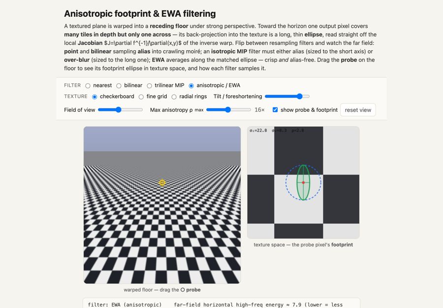
`fig-ewa-warp-demo` · **interactive** anisotropic resampling / EWA (6.2): a receding checkerboard floor compared under nearest / bilinear / trilinear-MIP / EWA filtering, with a draggable probe whose back-projected footprint ellipse is drawn in texture space — shows why an isotropic filter over- or under-blurs a stretched footprint ✅

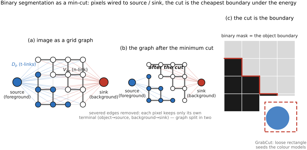
`fig-segmentation-graphcut` · binary segmentation as a min-cut on a grid graph wired to source/sink terminals; the cut is the object boundary (GrabCut inset) 🟨

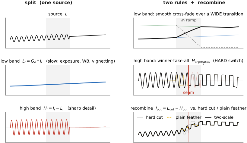
`fig-blend-twoscale-split` · a source split into low and high bands, the low band blended smoothly and the high band composited winner-take-all, plus a hard-cut / feather / two-scale comparison 🟨

⬜ figure not yet created

GrabCut rectangle → mask)

⬜ figure not yet created

`fig-graphcut-segmentation-demo` (**interactive** — scribble/rectangle graph-cut segmenter with a $\lambda$ smoothness slider and the live min-cut mask) fig-graphcut-segmentation-demo

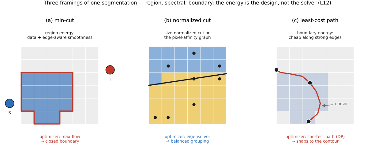
`fig-segmentation-three-framings` · three framings of segmentation — min-cut, normalized-cut, and least-cost path (intelligent scissors) — on the same boundary 🟨

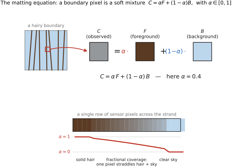
`fig-matting-equation` · the matting equation — one boundary pixel is $\alpha F + (1-\alpha)B$: a foreground color, a background color, and a soft coverage $\alpha$ 🟨

⬜ figure not yet created

`fig-trimap-to-alpha` (user trimap FG/BG/unknown → recovered continuous $\alpha$ over the unknown band) fig-trimap-to-alpha

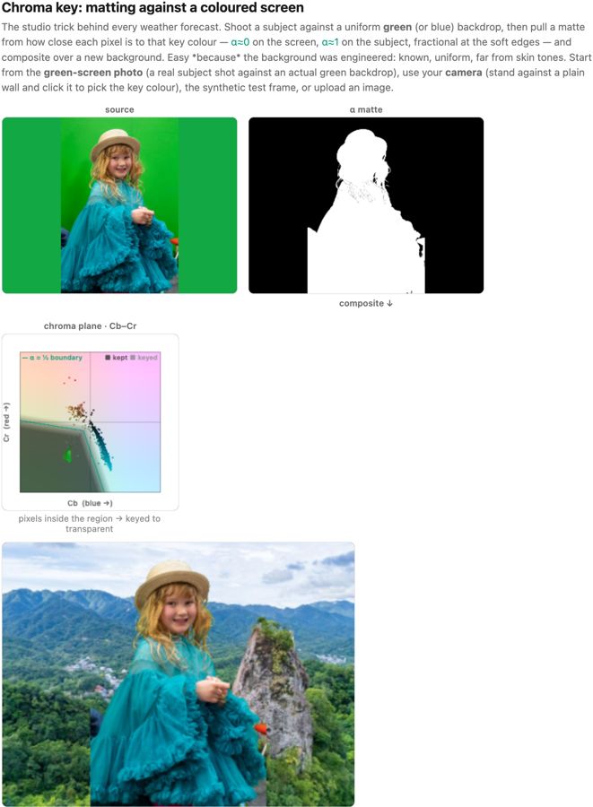
`fig-chroma-key` · **interactive** green/blue-screen matting (8.9, camera-capable): pull an $\alpha$ matte from color distance to the key (green/blue/eyedropped), tune tolerance/softness/spill, composite over a new background; source = built-in green-screen frame, upload, or live webcam ✅

⬜ figure not yet created

`fig-harmonization` (a correct-$\alpha$ cutout pasted raw ("stickered on") vs Poisson-blended vs color/lighting-harmonized → "belongs") fig-harmonization

The previous chapters fixed *one* image — denoise, deblur, recover detail. Now we **combine** images: separate a subject (above all a **person**) from its background and lay it over another. This is the most-used and least-solved editing operation — it drives portrait-mode **fake depth of field**, sky replacement, green-screen VFX, "select subject" — and it is still an **open problem**: even learning and generative methods are not quite there, partly because true mattes are nearly impossible to measure (training leans on **synthetic composites**). The chapter goes **compositing → segmentation → matting**: the forward, easy `over` operator and the alpha channel (the data model of Photoshop's layer stack) first, then the binary cut, then the soft one. The honest twist is that "which pixels are the subject" has no crisp answer at hair, fur, motion blur and glass — so the right object is not a binary mask but a **soft $\alpha$**, governed by one line, $C = \alpha F + (1-\alpha)B$, which is both ill-posed *and* non-linear.

equations

**compositing / matting equation** $C = \alpha F + (1-\alpha)B,\ \alpha\in[0,1]$ — *forward* = composite, *inverse* = matting (under-determined: 3 knowns, 7 unknowns per pixel)

**graph-cut segmentation energy** $E(\mathbf{L}) = \sum_p D_p(L_p) + \lambda \sum_{(p,q)\in\mathcal N} V_{pq}(L_p,L_q)$ with **data term** $D_p$ (color fit FG vs BG) and **edge-aware smoothness** $V_{pq}\propto \exp(-\lVert C_p-C_q\rVert^2/2\sigma^2)$ (an **affinity**, **L4.21**), minimized **exactly** for two labels by min-cut/max-flow (**L6.4**)

**closed-form matting** $\hat\alpha = \arg\min_\alpha \alpha^\top L\,\alpha$ s.t. trimap, where $L$ is the **matting Laplacian** (a pixel-affinity matrix from a local color-line model) — *the same affinity-Laplacian as colorization*

▸19.1.1 Compositing and alpha channels⧉

• **the `over` operator** (Porter & Duff 1984): a foreground carries a 4th channel $\alpha$, and over a background is the per-pixel $C=\alpha F+(1-\alpha)B$. $\alpha$ = **fractional coverage** — what fraction of the pixel the foreground occupies (or its opacity); $1$ inside, $0$ outside, **fractional at the boundary** (the point of antialiased / soft edges).

• **premultiplied (associated) alpha**: store color already scaled by coverage, $F'=\alpha F$, so over is $C=F'+(1-\alpha)B$. *Not* just cheaper — it is the representation under which **filtering/resampling is correct**: filtering *straight* alpha averages barely-covered pixels' full colors → **halos / fringes** ("black halo"); premultiplied filters color+coverage in lockstep → clean. Un-premultiply ($F=F'/\alpha$) only when you need true color; guard $\alpha=0$. [`fig-premultiplied-alpha-demo`]

• **the deeper connection**: this is the **bilateral grid**'s bookkeeping (store $\sum w_i v_i$ alongside $\sum w_i$, divide at slice — [[Bilateral filtering]]) and **homogeneous coordinates**' "carry $(wx,wy,w)$, divide by the last coord." Premultiplied alpha = $(\alpha R,\alpha G,\alpha B,\alpha)$ with the un-premultiply as the homogeneous divide. (Forward-ref added in the projective-geometry chapter, [[Pinhole image formation and linear perspective]].)

• **layers & blend modes**: a document is a **stack of layers** (color + alpha) composited bottom-to-top by repeated over — the non-destructive model of **Photoshop / After Effects**. **Blend modes** (multiply, screen, add, overlay, difference, …) swap a different per-pixel combine for plain over. File formats: **JPEG has no alpha**; **PNG / TIFF / PSD / OpenEXR** (premultiplied, multi-channel) carry it.

• **set up the inverse**: **segmentation** recovers a **binary** $\alpha$ (0/1 mask); **matting** recovers the **continuous** $\alpha\in[0,1]$ that segmentation can't represent.

▸19.1.2 Harmonization and where the blends live⧉

• **after a perfect cut, it can still look "stickered on"** — wrong light, white balance, contrast, grain. Matte right, *appearance* wrong. [`fig-harmonization`]

• **seamless blending**: **Poisson / gradient-domain** (Pérez et al. 2003 — paste gradients, re-derive boundary color; **L6.3**, [[Poisson image editing]]); **pyramid / multi-band** (Burt & Adelson 1983, [[Pyramids and wavelets]]). **Harmonization**: match color distribution / lighting / contrast / grain (Reinhard et al. 2001; learned). Poisson hides the **seam**, not a wrong **shading direction** — need all three: cut + blend + appearance.

• **the map**: **interactive digital photomontage** (Agarwala et al. 2004) wires both halves — a **graph-cut seam** (L6.4) picks the source per region, a **Poisson blend** (L6.3) hides it. **Multi-image fusion** (HDR / exposure fusion / focus stacking) → [[Multiple exposure imaging]] (combines exposures/focus, not objects). One line: **matting = the cut (here); Poisson/pyramid/photomontage = the blend (EDGES MATTER); HDR/fusion = the multi-capture combine.**

▸19.1.3 Optical effects beyond alpha⧉

• the **C = αF + (1−α)B** coverage model fails for **refractive/specular** foregrounds (glass, water, lenses): a pixel's color comes from *elsewhere* in the environment, bent and tinted, not the point behind it. **Environment matting** (Zongker et al. 1999) replaces the single α with a per-pixel **light-transport descriptor** (which background regions contribute + reflect/attenuate), captured via **structured backdrops** (Gray codes) — re-composite a glass over a new scene and it actually refracts it. Chuang et al. 2000: higher accuracy + real-time/video. Turns the per-pixel unknown from one coverage number into a slice of light transport → bridges to [[Computational illumination]].

▸19.2 Segmentation⧉

⬜ figure not yet created

`fig-premultiplied-alpha-demo` (**interactive** — filter a transparent cutout two ways: straight RGB (haloed/fringed) vs premultiplied (clean) fig-premultiplied-alpha-demo

⬜ figure not yet created

GrabCut rectangle → mask)

⬜ figure not yet created

`fig-graphcut-segmentation-demo` (**interactive** — scribble/rectangle graph-cut segmenter with a $\lambda$ smoothness slider and the live min-cut mask) fig-graphcut-segmentation-demo

⬜ figure not yet created

`fig-trimap-to-alpha` (user trimap FG/BG/unknown → recovered continuous $\alpha$ over the unknown band) fig-trimap-to-alpha

⬜ figure not yet created

`fig-harmonization` (a correct-$\alpha$ cutout pasted raw ("stickered on") vs Poisson-blended vs color/lighting-harmonized → "belongs") fig-harmonization

equations

**compositing / matting equation** $C = \alpha F + (1-\alpha)B,\ \alpha\in[0,1]$ — *forward* = composite, *inverse* = matting (under-determined: 3 knowns, 7 unknowns per pixel)

▸19.2.1 Segmentation: cutting the object out⧉

• **the task**: a **binary mask**. Three classic framings, one lesson (**L6.4**) — the energy/affinity you pick is the design, not the solver.

• **interactive graph-cut** (Boykov & Jolly 2001): grid graph + a few **FG/BG** strokes → a color **data term** $D_p$ + **edge-aware affinity** $V_{pq}\propto e^{-\lVert C_p-C_q\rVert^2/2\sigma^2}$; minimize $E=\sum_p D_p+\lambda\sum_{pq}V_{pq}$ by **min-cut/max-flow** — **globally optimal** for two labels. [`fig-segmentation-graphcut`] [`fig-graphcut-segmentation-demo`]

• 💡 **Big lesson (L6.4 + L4.21)**: a hard selection *is* the graph cut of [[Seam optimization]] — region data term + edge-aware smoothness, globally optimal for two labels; the optimizer is off-the-shelf, **choosing the energy is the design**. And $V_{pq}$ is an **affinity** (**L4.21**) — "how much these pixels belong together," now deciding *where not to cut*. The same affinity returns below as the **matting Laplacian**. (→ **L6.4** [[Seam optimization]], extending **L4.21** [[Bilateral filtering]].)

• **GrabCut** (Rother et al. 2004): a **loose rectangle** seeds Gaussian-mixture color models, run the cut, **re-estimate**, **iterate** — the interaction "select subject" descends from.

• **two other framings**: **normalized cuts** (Shi & Malik 2000, spectral — eigenvector of the graph Laplacian, unsupervised) and **intelligent scissors / live-wire** (Mortensen & Barrett 1995, least-cost path snapping to edges). Region / spectral / boundary — one **L6.4**. [`fig-segmentation-three-framings`]

• **the discrete sibling of colorization**: same energy (hard constraints + affinity smoothness) as [[Colorization]], but over a **binary** label (→ min-cut) rather than a **continuous** one (→ sparse linear solve). Matting relaxes the label back to continuous.

• **bridge to soft selection**: a hard 0/1 mask through **hair** looks scissor-cut — relax to a **continuous $\alpha$**.

▸19.3 Blue and green screen matting, chroma key⧉

⬜ figure not yet created

`fig-premultiplied-alpha-demo` (**interactive** — filter a transparent cutout two ways: straight RGB (haloed/fringed) vs premultiplied (clean) fig-premultiplied-alpha-demo

⬜ figure not yet created

GrabCut rectangle → mask)

⬜ figure not yet created

`fig-graphcut-segmentation-demo` (**interactive** — scribble/rectangle graph-cut segmenter with a $\lambda$ smoothness slider and the live min-cut mask) fig-graphcut-segmentation-demo

⬜ figure not yet created

`fig-trimap-to-alpha` (user trimap FG/BG/unknown → recovered continuous $\alpha$ over the unknown band) fig-trimap-to-alpha

⬜ figure not yet created

`fig-harmonization` (a correct-$\alpha$ cutout pasted raw ("stickered on") vs Poisson-blended vs color/lighting-harmonized → "belongs") fig-harmonization

equations

**compositing / matting equation** $C = \alpha F + (1-\alpha)B,\ \alpha\in[0,1]$ — *forward* = composite, *inverse* = matting (under-determined: 3 knowns, 7 unknowns per pixel)

▸19.3.1 Blue/green-screen matting and chroma keying⧉

• **the trick**: make $B$ **known by construction** — a uniform, saturated **green/blue screen** far from skin/hair → 3 unknowns gone, $\alpha B$ no longer an unknown product, the per-pixel solve for $\alpha,F$ is stable. **Chroma keying** (Smith & Blinn 1996; the Vlahos / Ultimatte lineage). [`fig-chroma-key`]

• **green vs blue**: **green** dominates (two green Bayer photosites → least-noisy channel; rarer in skin/wardrobe); **blue** was the film standard.

• **failure modes = ways "known $B$" breaks**: **spill** (screen bounce → de-spill), **uneven screen lighting** (why studios light it flat), **genuinely soft hair** (still must be matted). Moral: **chroma key removes unknowns by controlling the scene.**

• **the complementary road** — *measure* the FG/BG separation (depth / IR / flash falloff) rather than constrain $B$ — is [[Illumination-based matting]] (and is what portrait-mode depth seeds).

▸19.4 Matting⧉

⬜ figure not yet created

`fig-premultiplied-alpha-demo` (**interactive** — filter a transparent cutout two ways: straight RGB (haloed/fringed) vs premultiplied (clean) fig-premultiplied-alpha-demo

⬜ figure not yet created

GrabCut rectangle → mask)

⬜ figure not yet created

`fig-graphcut-segmentation-demo` (**interactive** — scribble/rectangle graph-cut segmenter with a $\lambda$ smoothness slider and the live min-cut mask) fig-graphcut-segmentation-demo

⬜ figure not yet created

`fig-trimap-to-alpha` (user trimap FG/BG/unknown → recovered continuous $\alpha$ over the unknown band) fig-trimap-to-alpha

⬜ figure not yet created

`fig-harmonization` (a correct-$\alpha$ cutout pasted raw ("stickered on") vs Poisson-blended vs color/lighting-harmonized → "belongs") fig-harmonization

equations

**compositing / matting equation** $C = \alpha F + (1-\alpha)B,\ \alpha\in[0,1]$ — *forward* = composite, *inverse* = matting (under-determined: 3 knowns, 7 unknowns per pixel)

▸19.4.1 The fundamental matting equation⧉

• **the inverse**: see only $C$ (3 numbers), recover $F$ (3), $B$ (3), $\alpha$ (1) — **7 unknowns, 3 equations** per pixel. [`fig-matting-equation`]

• 💡 **Big lesson — matting is non-linear**: unlike the linear forward models of [[Image formation as a linear system]] / 2.10, the term $\alpha F$ **multiplies two unknowns** — bilinear, not linear, so there is no $A$ with $C=A(\alpha,F,B)$. Matting is doubly hard: **under-determined *and* non-linear**. Every method either *fixes some unknowns* (so the rest is linear) or *biases hard* with a prior/learning. (Extends **L5.4** · the prior is not optional, [[#Super-resolution]].)

• **the four-rung ladder of extra knowledge**: (1) **known background** (chroma key — $B$ known, which removes three unknowns but still leaves four per pixel against three equations, so it needs a color assumption or a second background to be determined); (2) a **trimap**; (3) an **inductive bias** about local color (Bayesian / Laplacian); (4) **learning** (and generative priors).

• **the trimap**: three-way label — definitely FG / definitely BG / a thin **unknown band $\Omega$**. In the definite regions $\alpha$ is pinned and $F$ or $B$ is *observed*; solve only the narrow band with nearby colors as anchors. Less input is the arc: scribble → rectangle → trimap → **nothing**. [`fig-trimap-to-alpha`]

▸19.4.2 Traditional matting approaches⧉

• honesty: now **dominated by learning**; these two survive as the clearest way to *feel* the problem.

• **Bayesian matting** (Chuang et al. 2001): per-pixel **MAP** — model nearby FG/BG colors as Gaussians, find the $(F,B,\alpha)$ best explaining $C$, sweep outward. Shows how *ambiguous* the problem is; **local** (neighboring alphas needn't agree → noisy).

• **closed-form / Laplacian matting** (Levin, Lischinski & Weiss 2008; refresher from [[Matting Laplacian]]): assume FG/BG lie on local **color lines** → $\alpha$ is locally **affine in color**, which **eliminates $F,B$ and the non-linearity**, leaving $\hat\alpha=\arg\min_\alpha\alpha^\top L\alpha$ s.t. trimap — a **sparse linear solve**.

• 💡 **the hinge (L4.21)**: $L$ **plays the role of an affinity Laplacian**, like the bilateral weight, the graph-cut $V_{pq}$ and the **colorization** solve (the same authors' 2004 work), but its weights come from a local color-line model fitted in each window rather than from a pairwise color distance, and some can be negative. Its color-line energy captures local image correlations so well it travels far (dehazing-transmission refinement, guided filtering, inside learned matting). (→ **L4.21** [[Bilateral filtering]].)

• **robust / sampling hybrids** (Wang & Cohen 2007): color-sampling + affinity smoothness — the workhorse just before learning.

▸19.4.3 Deep-learning matting⧉

• 💡 **callback to L5.3**: same skeleton (recover $\alpha$), swap the hand-built prior for a function **fit to data** — learns the *appearance* of hair/fur/blur, inherits data-dependence.

• **Deep Image Matting** (Xu et al. 2017): **image + trimap → encoder–decoder** regresses $\alpha$ (+ refinement net), alpha loss + **compositing loss**. Introduced **Composition-1k** — hundreds of real foregrounds × thousands of backgrounds = synthetic composites (the field's enabling trick *and* original sin).

• **trimap-free**: **MODNet** (Ke et al. 2022 — *queue ref*) predicts a portrait matte from the image alone, real-time; **background matting** (Sengupta et al. 2020 — *queue ref*; real-time HD: Lin et al. 2021) takes one extra **clean-plate** photo — a hand-held descendant of chroma key powering video-call backgrounds.

• **video**: **temporal coherence** (flicker looks worse than stable error → track / flow-warp the matte) — the learned successor to hand **rotoscoping**.

• **the limited-data ceiling** (tie back to intro): real mattes are nearly unmeasurable → training is mostly **synthetic composites**, so nets learn that pipeline's statistics — brittle on real snapshots.

▸19.4.4 Generative matting⧉

• **SAM — Segment Anything** (Kirillov et al. 2023): promptable (point/box/"everything") → clean masks for arbitrary objects, no per-class training; collapses GrabCut to one prompt. But **binary** — segmentation, not matting.

• **SAM-driven matting**: **Matte Anything** (Yao et al. 2024 — *queue ref*) — SAM mask → auto-trimap → matting net (one-prompt, trimap-free).

• **diffusion priors**: **diffusion-based matting** (DiffMatte etc. — *queue ref*) conditions a generative image model ([[Generative AI and diffusion]]) to *denoise toward* a plausible matte — richer world-knowledge than a color line or a small dataset.

• **why still short**: generative priors **hallucinate plausible, not correct** hair (the SR forensic caveat); and they are still calibrated on the same scarce, mostly-synthetic data → inherit its blind spots. Matting stays an **open problem**; roto artists not yet retired.