BookNotesSlidesP-sets Syllabusdraft · v0.2.49.1
💬Comments welcome. To leave a note, select any text and click the note / highlight button that pops up — or open the panel with the tab at the top-right (‹). Notes are visible only inside our private review group.
Computational Photography, an AI-powered Slopendium — 13 Denoising
expand to📖 Full book outline1 parts · 14 chapters · 62 sections · 17 figures embedded · 10 placeholders · double-click a figure to enlarge
▸Part 13 DENOISING⧉
<!--uid: denoising-part-->
▸13.1 Noise models, transforms, and benchmarks⧉
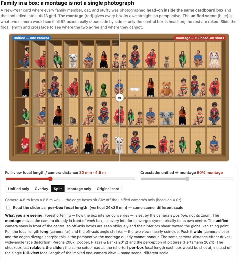
fig-perspective-montage
fig-perspective-montage · "family in a box" New-Year-card demo (real 3D): a 4×13 grid of cardboard boxes, each holding a diverse family member / cat / stuffy, rendered two ways and overlaid — the **montage** (every box shot head-on, its own perspective) vs. the **unified scene** (one camera in front of the center, edge boxes raked toward the global vanishing point); focal-length / distance slider + crossfade show the two coincide at long focal length and diverge wide. After [Durand, *Family in a box* (2023)](https://www.thecomputationalphotographer.net/2023/01/family-in-a-box/); perspective-perception refs Cooper-Piazza-Banks 2012, Hertzmann 2024. *Human, cat & stuffy 3D models generated with Meshy AI.* ✅
equations
$y = x + n$
the affine variance law
the Anscombe transform $f(y) = 2\sqrt{y + 3/8}$ and its exact unbiased inverse
PSNR and SSIM as the reported numbers, with their known failure modes ([[Image metrics]]).
13.1.1 The noise that is actually there⧉
13.1.2 Choosing the working domain⧉
13.1.3 Variance-stabilizing transforms⧉
13.1.4 A ladder of difficulty⧉
13.1.5 Salt-and-pepper is a different problem⧉
13.1.6 Benchmarks, and what a leaderboard number means⧉
▸13.2 Denoising by averaging⧉
⬜ figure not yet created
`fig-averaging-N-frames` (one noisy frame → mean of 3 → mean of 5 → mean of 45: the gray patch's histogram visibly narrows, after the Canon-1D ISO-3200 slide sequence) fig-averaging-
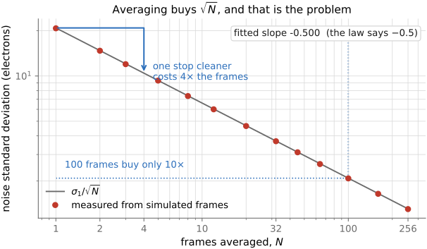
fig-sqrt
fig-sqrt ·
⬜ figure not yet created
doubling cleanliness costs 4× the frames)
⬜ figure not yet created
`fig-iid-variance-adds` (schematic of the derivation: $N$ independent noise samples, variance adds then $\div N^2$ → $\sigma^2/N$) fig-iid-variance-adds
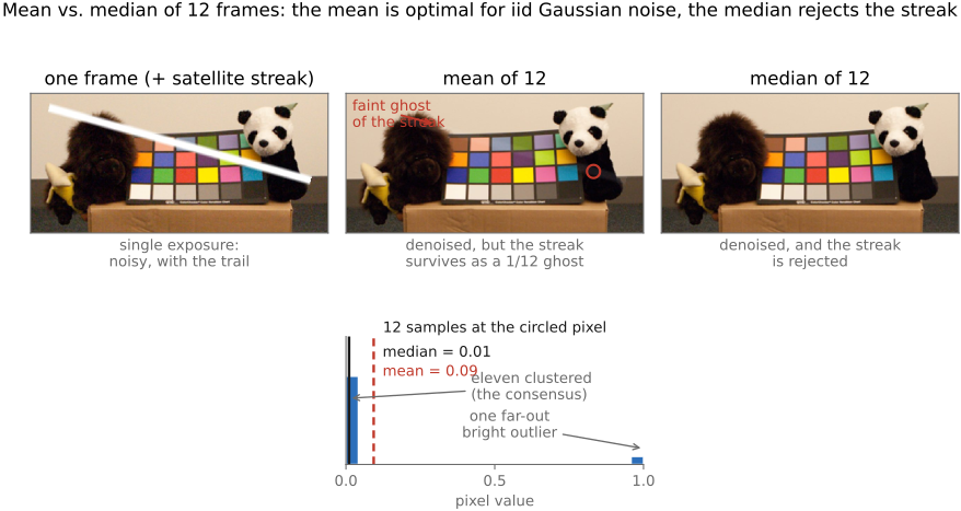
fig-mean-vs-median-stack
fig-mean-vs-median-stack · plain-mean stack (residual ghost streak from one outlier frame) vs median / sigma-clip stack (streak rejected) of the same frames, with the per-pixel sample distribution inset ✅
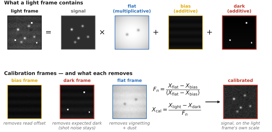
fig-calibration-triad
fig-calibration-triad · a light frame's bias / dark / flat components and the calibration formula $X_\text{cal}=(X_\text{light}-X_\text{dark})/(X_\text{flat}-X_\text{bias})$ that subtracts the additive terms and divides out the multiplicative one 🟨
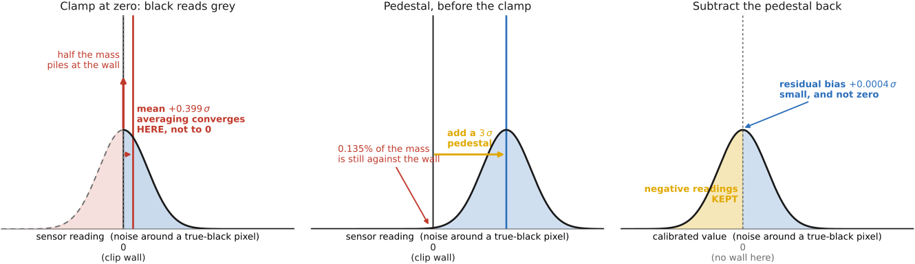
fig-clipping-bias
fig-clipping-bias · how clamping noise at zero biases a dark region bright under averaging, and how a pre-read positive offset restores zero-mean behavior 🟨
⬜ figure not yet created
`fig-astro-stack-reveal` (a single 30-s sub of a faint galaxy — almost noise — vs 200 subs stacked: structure emerges) fig-astro-stack-reveal
⬜ figure not yet created
`fig-sub-length-tradeoff` (read-noise floor vs total integration time: fewer-longer beats more-shorter once read noise is sub-dominant) fig-sub-length-tradeoff
💡 **Big lesson (the $1/\sqrt N$ law — averaging $N$ independent measurements halves the noise every 4× frames):** model each pixel as a true value plus **independent, zero-mean** noise. Averaging $N$ frames leaves the true value alone (its average is the true value) but the **noise variance falls as $1/N$**, so the **standard deviation — the visible error — falls as $1/\sqrt N$**. This is the part's recurring quantitative result: it is the same law behind HDR's noise-weighted merge, burst low-light (HDR+ / Night Sight), burst super-resolution, and astrophotography's hours of integration. The diminishing-returns sting is built in — *each extra stop of cleanliness costs four times the frames*. (It ties to **L2.48** — averaging is the algorithmic way to lower the effective **noise floor**, the complement to widening the well; the two together set how much real signal you can pull from shadow. Registered in [[Big Lessons]] alongside L2.48; first developed here.)
💡 **Big lesson (L11.2 · capture the full set, decide later):** rather than commit at the instant of exposure, **record the whole set and choose afterward**. Averaging is the first instance in this part: don't take *one* careful frame and hope — take a **burst** and combine. The same move recurs as exposure bracketing (capture all exposures → [[#HDR merging]]), focus stacks (capture all focal planes), and panoramas (capture all directions). The cost is data and a reconstruction step; the payoff is deferring an irreversible decision out of the moment of capture. (Registered in [[Big Lessons]] as **L11.2**; this part is its natural home.)
The previous part measured and characterized noise. This part *fights* it — and the bluntest, most trustworthy weapon is to take the **same picture many times and average**. No prior, no model of what images look like: just repeated measurement and the law of large numbers. Where single-image denoising ([[Bilateral filtering]]) must *guess* which neighbors to trust, averaging multiple frames adds **genuine independent information** with each shot. The whole chapter is one derivation and its consequences.
equations
noise model per pixel per frame $X_i = \mu + n_i$, with $\mathbb{E}[n_i]=0$ (zero-mean) and $\operatorname{Var}[n_i]=\sigma^2$, the $n_i$ **independent** across frames
the average $\bar X = \tfrac1N\sum_{i=1}^N X_i$
**unbiased** in the signal $\mathbb{E}[\bar X]=\mu$
the two variance rules $\operatorname{Var}[kX]=k^2\operatorname{Var}[X]$ and (independence) $\operatorname{Var}\big[\sum_i X_i\big]=\sum_i\operatorname{Var}[X_i]$
hence $\operatorname{Var}[\bar X]=\tfrac{1}{N^2}\cdot N\sigma^2=\dfrac{\sigma^2}{N}$, so $\boxed{\sigma_{\bar X}=\dfrac{\sigma}{\sqrt N}}$
sample-variance estimator with **Bessel correction** $\hat\sigma^2=\tfrac{1}{N-1}\sum_i (X_i-\bar X)^2$ (divide by $N{-}1$, not $N$ — removes the downward bias from reusing the same samples for mean and variance)
SNR $=\mu/\sigma$, in dB $20\log_{10}(\mu/\sigma)$, improving by $10\log_{10}N$ ($\approx 3$ dB per doubling)
calibration $\
X_\text{cal}=\dfrac{X_\text{light}-X_\text{dark}}{X_\text{flat}-X_\text{bias}}$ (subtract additive fixed-pattern, divide out multiplicative).
13.2.4 Handheld low light: the phone in your pocket⧉
13.2.6 When is splitting the light free?⧉
▸13.3 Gaussian, median, and bilateral filtering⧉
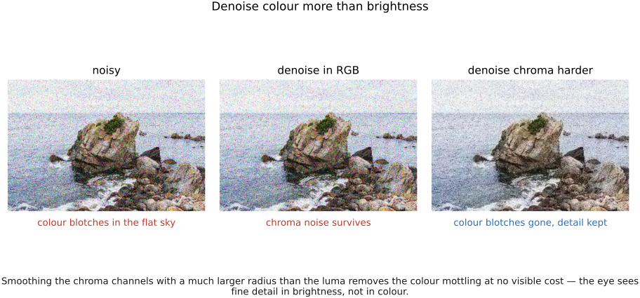
fig-denoise-chroma
fig-denoise-chroma · denoise color more than brightness: noisy real crop vs RGB denoise (chroma noise survives) vs luma/chroma denoise (aggressive chroma blur kills color blotches, keeps detail) (Denoising, BASIC) ✅
equations
the Gaussian kernel
the bilateral weight $w(p,q) = G_{\sigma_s}(\lVert p-q\rVert)\,G_{\sigma_r}(\lvert I_p - I_q\rvert)$.
13.3.1 Gaussian smoothing, and the assumption inside it⧉
13.3.2 The median, and the noise it is actually for⧉
13.3.3 The bilateral filter: a neighborhood that looks at the pixels⧉
13.3.4 Denoise color more than brightness⧉
13.3.5 What each filter destroys⧉
13.3.6 The noise these filters were shown with, and the noise a sensor makes⧉
13.3.7 Filtering in a stabilized domain⧉
13.3.8 Or vary the widths instead⧉
▸13.4 Pyramid and wavelet denoising⧉
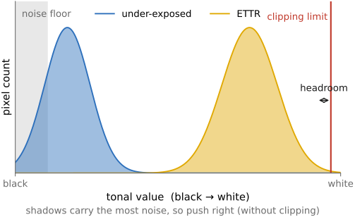
fig-ettr-histogram
fig-ettr-histogram · expose-to-the-right: an image histogram pushed toward the highlights without clipping (vs an under-exposed one bunched at the noise floor) 🟨
equations
soft threshold $\operatorname{sign}(c)\max(|c|-\lambda, 0)$
the universal threshold $\lambda = \sigma\sqrt{2\log N}$.
13.4.1 Sparse in the right basis⧉
13.4.2 Thresholding, hard and soft⧉
13.4.3 Shrinkage as a MAP estimate⧉
13.4.4 Ringing, and why the transform is usually overcomplete⧉
13.4.5 Coring band by band, in practice⧉
13.4.6 Coring and the Gaussian scale mixture⧉
▸13.5 Total variation and optimization-based denoising⧉
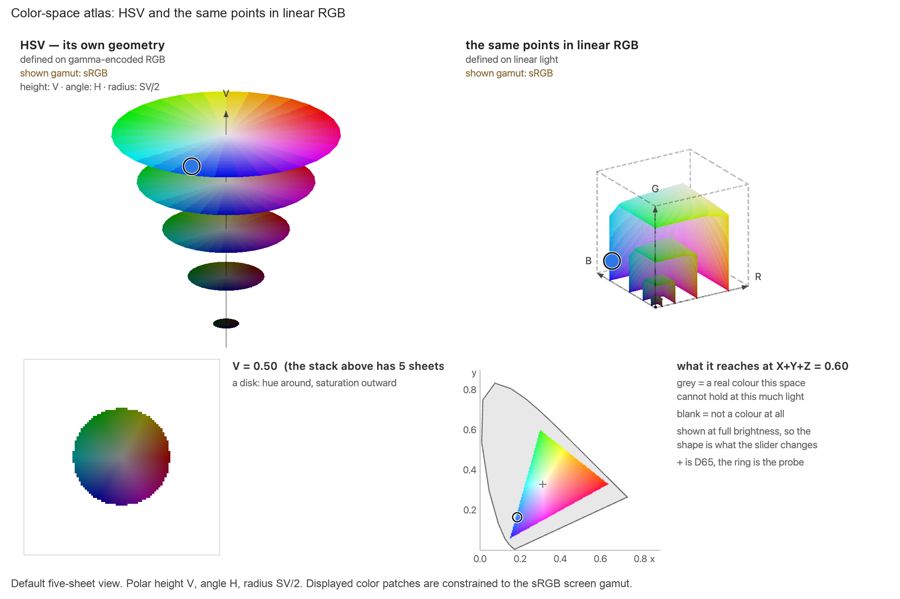
fig-color-space-atlas
fig-color-space-atlas · **interactive** color-space atlas: one space drawn twice, in its own geometry (cube / cone / bi-cone / warped cube) and in a chosen ambient frame (XYZ, LMS, linear RGB, sRGB, Chong, Oklab), from the same lattice, as edges / voxels / one slice; MacAdam ellipses optional; click to read coordinates in both; stripes for colors outside sRGB. Placed at the end of the perceptually-uniform section of **4.6 Advanced color**, where it works as the chapter's capstone: by then HSV/HSL, CIELAB, Oklab and Chong have each been shown alone, and the atlas is about the map between them. URL carries the state (`?space=&ambient=&mode=&axis=&at=&grid=&macadam=&zebra=`). 🟨
fig-lens-design-tradeoff
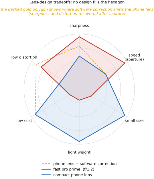
fig-lens-design-tradeoff · lens-design Pareto cartoon as a 6-axis radar (sharpness, speed, size, weight, cost, distortion): fast pro prime vs compact phone lens overlaid, plus a dashed polygon showing where software correction shifts the phone lens (Lens optimization) ✅
equations
the ROF objective
the two penalties on a step edge, worked
one ADMM iteration with the TV proximal step named.
13.5.1 Why the penalty's shape decides the answer⧉
13.5.2 Isotropic, anisotropic, and the staircase⧉
13.5.3 Solving it⧉
13.5.4 Where it stands now⧉
▸13.6 Non-local means and BM3D⧉
fig-ssim-map
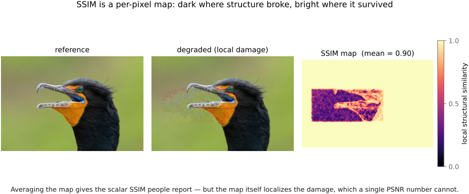
fig-ssim-map · SSIM as a per-pixel map: reference, locally-damaged copy (one band JPEG-blocked + noised), and the SSIM heat-map that goes dark exactly on the damage — its mean is the scalar SSIM (Image metrics, BASIC) ✅
⬜ figure not yet created
a BM3D patch stack drawn as the 3-D group it is.
equations
the NL-means weight $w(p,q) \propto \exp(-\lVert P_p - P_q\rVert^2/h^2)$.
13.6.1 A photograph repeats itself⧉
13.6.2 Non-local means: similarity as the weight⧉
13.6.3 BM3D: group, transform, shrink, aggregate⧉
13.6.4 The ceiling of hand-designed priors⧉
▸13.7 Learned denoisers⧉
fig-ettr-histogram
fig-ettr-histogram · expose-to-the-right: an image histogram pushed toward the highlights without clipping (vs an under-exposed one bunched at the noise floor) 🟨
⬜ figure not yet created
the unrolling diagram, iterations drawn as layers.
equations
the residual objective $\lVert \mathcal N(y) - (y - x)\rVert^2$
one ISTA step, then the same step with learned parameters.
13.7.1 DnCNN: learn the noise, not the image⧉
13.7.2 FFDNet: hand the network the noise level⧉
13.7.3 DRUNet: a denoiser built to be reused⧉
13.7.4 Unrolling: from learning a function to learning an algorithm⧉
▸13.8 Denoising without clean data⧉
⬜ figure not yet created
the assumption ladder as one table, requirement against method fig-uxr-method-definitions
fig-seidel-aberrations
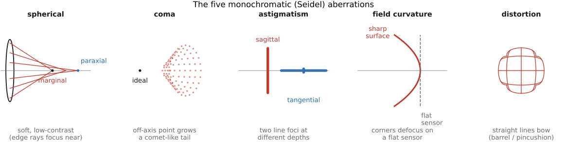
fig-seidel-aberrations · the five monochromatic (Seidel) aberrations at a glance — spherical, coma, astigmatism, field curvature, distortion — each a tiny ray/spot icon + a one-line "what it looks like" note ✅
13.8.1 CBDNet: estimate the noise, keep the pairs⧉
13.8.2 Noise2Noise: two noisy observations⧉
13.8.3 Noise2Void and Noise2Self: one noisy image⧉
13.8.4 Blind2Unblind: recovering information hidden by the blind spot⧉
13.8.5 Choosing supervision for a real camera⧉
▸13.9 Generative denoising with diffusion models⧉
fig-denoising-without-prior
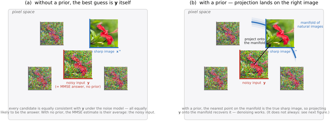
fig-denoising-without-prior · (a) noisy image + Gaussian cloud of consistent clean images (no prior); (b) add manifold (high curvature) — noisy point off it, MMSE/posterior-mean of two sharp on-manifold images lands off-manifold & blurry ("average is dull") ✅
13.9.1 Why the posterior mean can blur detail⧉
13.9.2 Sampling instead of averaging⧉
13.9.3 The reverse process is a sequence of denoisings⧉
13.9.4 What a hallucinated detail costs⧉
▸13.10 Video denoising⧉
⬜ figure not yet created
a flicker figure that only works in motion, one noisy clip denoised per frame and denoised temporally, played side by side fig-reduce-over-time
fig-color-space-atlas
fig-color-space-atlas · **interactive** color-space atlas: one space drawn twice, in its own geometry (cube / cone / bi-cone / warped cube) and in a chosen ambient frame (XYZ, LMS, linear RGB, sRGB, Chong, Oklab), from the same lattice, as edges / voxels / one slice; MacAdam ellipses optional; click to read coordinates in both; stripes for colors outside sRGB. Placed at the end of the perceptually-uniform section of **4.6 Advanced color**, where it works as the chapter's capstone: by then HSV/HSL, CIELAB, Oklab and Chong have each been shown alone, and the atlas is about the map between them. URL carries the state (`?space=&ambient=&mode=&axis=&at=&grid=&macadam=&zebra=`). 🟨
equations
the motion-compensated average $\hat x_t(\mathbf p) = \frac{1}{|\mathcal N|}\sum_{s \in \mathcal N} y_s(\mathbf p + \mathbf d_{s \to t}(\mathbf p))$
a temporal-consistency penalty on warped consecutive outputs.
13.10.1 Temporal redundancy is the resource⧉
13.10.2 Patches in space and time⧉
13.10.3 Learned video denoisers⧉
13.10.4 Temporal consistency, and the metric that does not measure it⧉
▸13.11 Denoising as a universal prior⧉
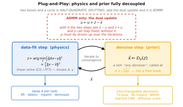
fig-pnp-loop
fig-pnp-loop · Plug-and-Play / RED: alternate a data-fidelity step with a denoiser-as-prior step until convergence — the prior is a black-box denoiser 🟨
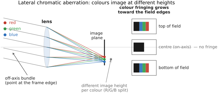
fig-lateral-chromatic
fig-lateral-chromatic · lateral (transverse) CA: an off-axis bundle where R/G/B image at different HEIGHTS (different magnification per color) on the common image plane → colored fringes growing toward the frame edge; inset of the fringed edge (distinct from axial CA) ✅
equations
the HQS or ADMM split with the proximal step named as a denoising problem
$\rho(x) = \tfrac12 x^{\mathsf T}(x - D(x))$ and $\nabla\rho(x) = x - D(x)$
Tweedie, $\mathbb E[x \mid y] = y + \sigma^2\nabla_y \log p(y)$.
13.11.1 Plug-and-play: a denoiser inside ADMM⧉
13.11.2 Reusing the denoiser across measurement models⧉
13.11.3 RED: the denoiser as an explicit regularizer⧉
13.11.4 Tweedie's formula, and what a denoiser has been computing⧉
13.11.5 Sampling with a denoiser-derived score⧉
13.11.6 DRUNet as a plug-and-play prior, and continuation⧉
▸13.12 Measuring a denoiser⧉
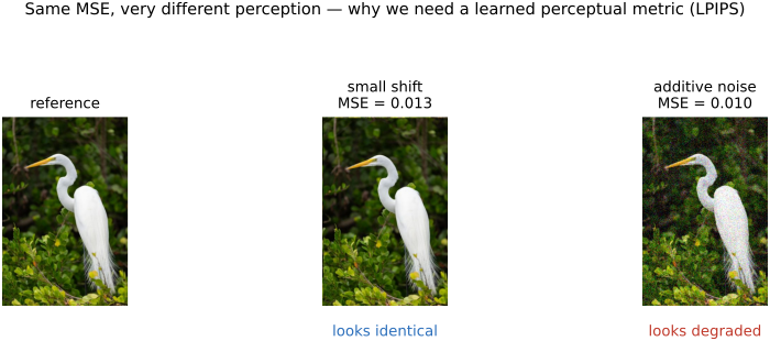
fig-perceptual-metric
fig-perceptual-metric · same MSE, very different perception (small shift vs additive noise) → why LPIPS (ML) ✅
⬜ figure not yet created
a quality-against-cost plot with real timings.
13.12.1 The reference metrics, and what each rewards⧉
13.12.2 Comparing operating points⧉
13.12.3 What to hold fixed⧉
13.12.4 Ablations, cost, and what to report⧉
13.12.5 The question a benchmark does not answer⧉
▸13.13 The limits of denoising⧉
• there's a floor: **Levin et al.** bound how much *any* denoiser can recover — once noise swamps the local structure, detail is unrecoverable; stronger **priors** (and more photons) are the only way past it
• 💡 **L4.22 — the average is safe, and the average is dull**: MMSE = the **mean** of all images consistent with the data; over genuine uncertainty that average is **blurry / washed-out**. *Two perspectives on why* — (1) **convexity / geometry**: the natural-image set is **non-convex**, so a convex average of two valid images falls **off the manifold** into the blurry gap (the manifold is messy); (2) **perception**: the squared-error ruler MMSE uses treats image space as **Euclidean**, but **human perception is not Euclidean in image space** (a global shift is $L_2$-huge yet perceptually trivial; wrong texture is $L_2$-tiny yet glaring) — so the metric is mismatched too. Escape = change the objective (perceptual/adversarial loss) or **sample** one sharp outcome (diffusion) instead of averaging.
• **side bar (ethics) — when denoising becomes beautification**: pushed too far, denoising (especially on **skin**) erases **texture** (pores, fine lines) → the **"plastic" / wax-figure** look; skin-smoothing, blemish-removal and **beautification** are the *same operation* dialled up (suppress high-freq variation in detected skin). Phones often apply it **by default**, non-consensually — silently imposing a flawless-skin standard, making the photo unfaithful to the person, and affecting **self-image** (esp. young people). Where does a denoiser stop cleaning an image and start editing a face? → ties to ethics ([[Human factors and the art of photography]])
13.14 Denoising TLDR⧉